Getting Started

Prediction-Based Inference: Methods & Applications

Build intuition for prediction-based inference by simulating data and comparing different methods.

Overview

Welcome to this workshop on Prediction-Based (PB) Inference.

In this first module, we use a simple synthetic example to build intuition for how PB inference works and why it is needed. We will:

Introduce the ipd package,
Generate synthetic labeled and unlabeled data,
Compare naive, classical, and PB estimators, and
Inspect results using built-in tidy(), glance(), and augment() methods.

Throughout the workshop, each exercise includes a solution and short notes to help connect the results back to the main PB inference ideas.

How to Use This Module

Try each Exercise on your own first.
Expand the Answer callout to view one possible solution.
Use the Notes callouts to interpret the results and connect them to the main concepts.

Why This Unit Uses Synthetic Data

Unit 00 uses synthetic examples on purpose. The goal is to make the PB inference workflow concrete before moving to real applications in later modules.

Key Takeaway

Using predicted outcomes can improve efficiency, but treating them as if they were the true observed outcomes can bias downstream inference. PB inference methods use a small labeled set to correct that bias while still borrowing information from unlabeled data and predictions.

In this unit, we will:

Generate synthetic data.
Fit simple downstream regression models.
Apply ipd::ipd() to estimate the association between Y and X1.
Compare naive, classical, and PB estimates.
Visualize uncertainty across methods.

Installation and Setup

First, make sure you have the ipd package and a few supporting packages installed:

Code

# Install these packages if you have not already:
# install.packages(c("ipd", "MASS", "broom", "tidyverse", "patchwork"))

library(ipd)
library(MASS)
library(broom)
library(tidyverse)
library(patchwork)

Throughout the workshop, we will use reproducible seeds and tidyverse conventions.

Function References

Here is a brief overview of the main ipd functions used in this unit.

`ipd()`

ipd() fits IPD estimators for downstream inference with predicted outcomes.

ipd(
  formula,      # A formula: e.g., Y - f ~ X1 + X2 + ...
  method,       # Character: one of "chen", "pdc", "postpi_analytic", 
                # "postpi_boot", "ppi", "ppi_all", "ppi_plusplus", "pspa"
  model,        # Character: one of "mean", "quantile", "ols", "logistic", 
                # "poisson"
  data,         # Data frame containing columns for formula and label
  label,        # Character: name of the column with set labels ("labeled" and 
                # "unlabeled")
  ...           # Additional arguments
)

Supported Methods

Methods currently implemented are:

chen: Chen and Chen Estimator (Gronsbell et al., 2026)
pdc: Prediction Decorrelated Inference (Gan et al., 2024)
postpi_analytic: Analytic Post-Prediction Inference (Wang et al., 2020).
postpi_boot: Bootstrap Post-Prediction Inference (Wang et al., 2020).
ppi: Prediction-Powered Inference (Angelopoulos et al., 2023)
ppi_plusplus: PPI++ (PPI with Data-Driven Weighting; Angelopoulos et al., 2024)
ppi_a: PPI using All Data (Gronsbell et al., 2026)
pspa: Assumption-Lean and Data-Adaptive Post-Prediction Inference (Miao et al., 2024)

Tidy Methods

Like many model objects in R, ipd fits work with familiar helper functions:

print() and summary(): display model summaries.
tidy(): return a tibble of estimates and standard errors.
glance(): return a one-row tibble of model-level metrics.
augment(): return the original data with fitted values and residuals.

Simulating Data

The ipd package provides a function for simulating data based on the approach in Wang et al. (2020). We provide more detail about this function at the end of this model. Here, we will be generating synthetic data following Gronsbell et al. (2026) and Ji et al. (2025) to better illustrate the core principles of PB inference in a more straightforward manner. We provide helper functions below to simulate data from a linear regression model.

#--- Function for the l2 Norm

l2_norm <- function(x, squared = FALSE) {
  
  y <- sum(x^2)
  
  if (!squared) {
    
    y <- sqrt(y)
  }
  
  return(y)
}

#--- Function to Generate from the Unit Sphere S^{d-1}

unit_vec <- function(d) {
  
  v <- rnorm(d)
  
  return(v / l2_norm(v))
}

#--- Function to Simulate Data

simple_data_gen <- function(
    n,                 # Number of Samples
    p = 2,             # Number of Covariates
    prop_lab = 0.1,    # Proportion of Labeled Observations
    total_var = 20,    # Total Variance
    ratio_var = 1,     # Variance Ratio
    rho = 0,           # Covariate Correlation
    sigma_y = 1,       # Outcome Error Variance
    beta = c(1,1),     # Effect Sizes
    predset_ind = 1) { # Indices for Covariates Used for Prediction.
  
  #- Covariate Covariance Matrix
  
  sigma_x <- total_var / (ratio_var + 1)
  
  sigma_w <- ratio_var * sigma_x
  
  cov_diag <- sqrt(c(rep(sigma_x, p / 2), rep(sigma_w, p / 2))) 
  
  cov_matrix <- (1 - rho) * diag(cov_diag^2) + rho * (cov_diag %o% cov_diag)
  
  #- Generate Covariates
  
  x <- MASS::mvrnorm(n, mu = rep(0, p), Sigma = cov_matrix)
  
  colnames(x) <- paste0('x', 1 : p)
  
  #- Generate Outcome
  
  eps <- rnorm(n, sd = sigma_y) 
  
  lin_pred <- x %*% beta 
  
  y <- lin_pred + eps
  
  #- Inference Data
  
  inference_data <- data.frame(y = y, x)
  
  #- Generate Predictions
  
  pred_covs <- as.matrix(inference_data[, paste0("x", predset_ind)])
  
  pred_beta <- c(beta[predset_ind])
    
  f <- pred_covs %*% pred_beta
  
  #- Analysis Data
  
  analysis_data <- data.frame(inference_data, f)
  
  samp_ind <- rbinom(n, 1, prop_lab)
  
  analysis_data$set_label <- ifelse(samp_ind == 1, "labeled", "unlabeled")
  
  return(as_tibble(analysis_data))
}

Exercise 1: Data Generation

Let us generate a synthetic dataset for a linear model with:

n = 25000 samples
p = 10 covariates
A prop_lab = 0.1 proportion of labeled observations
A total variance of total_var = 20
A variance ratio of ratio_var = 1
No covariate correlation (rho = 0)
A sigma_y = 5 outcome error variance
Coefficients beta <- c(unit_vec(p / 2), unit_vec(p / 2)) generated from the unit circle
predset_ind = 1 : 10 indices for covariates used for prediction

The first setting is an ‘ideal’ setting that mimics when the prediction is derived from a linear model that was estimated on a large, independent dataset with the same distribution of \(Y | X\) as the dataset used for conducting inference. Here, we generate predictions based on all \(X\)’s being available. In this stylized example, we are generating predictions \(f = E[Y | X]\) so the naive approach should be unbiased, but still anti-conservative, as we do not fully capture the variability of \(Y\).

Answer

set.seed(123)

n <- 25000 # Number of Samples
p <- 10    # Number of Covariates

b1 <- unit_vec(p / 2) # Effect Sizes
b2 <- unit_vec(p / 2)

dat_ipd <- simple_data_gen(
    n = n,               # Number of Samples
    p = p,               # Number of Covariates
    prop_lab = 0.1,      # Proportion of Labeled Observations
    total_var = 20,      # Total Variance
    ratio_var = 1,       # Variance Ratio
    rho = 0,             # Covariate Correlation
    sigma_y = 5,         # Outcome Error Variance
    beta = c(b1, b2),    # Effect Sizes
    predset_ind = 1:10  # Indices for covariates used for prediction.
)

# The resulting tibble `dat_ipd` has columns:
#  - X1, X2, ..., Xp: Simulated covariates 
#  - Y              : True outcome 
#  - f              : Predicted outcome 
#  - set_label      : {"labeled", "unlabeled"}

# Quick look:
dat_ipd |> 
  group_by(set_label) |> 
  summarize(n = n())

# A tibble: 2 × 2
  set_label     n
  <chr>     <int>
1 labeled    2551
2 unlabeled 22449

Let us also inspect the first few rows of each subset:

Answer

# Labeled set
dat_ipd |>
  filter(set_label == "labeled") |>
  glimpse()

Rows: 2,551
Columns: 13
$ y         <dbl> -10.6651305, 7.0229562, 1.8466360, 5.6049078, 4.4638744, -6.…
$ x1        <dbl> 2.8081938, 1.4447090, 1.1134905, 1.2321898, -0.2950160, 4.69…
$ x2        <dbl> -2.1727482, 1.1195759, 0.1438820, 4.8518833, -1.0137343, 4.4…
$ x3        <dbl> -7.07650307, 0.77112369, -0.01939504, -0.66786699, -4.538479…
$ x4        <dbl> 2.1733859, 3.8373017, 0.3445341, 1.6177814, -1.8449544, -3.7…
$ x5        <dbl> -0.5130663, 2.9121691, 5.2980682, 1.0774526, -1.0392365, -0.…
$ x6        <dbl> -4.32514921, 2.60046203, -0.06035815, -0.23868960, 6.9521900…
$ x7        <dbl> -0.75585286, 3.65797447, 5.16160001, 6.18270859, -4.01256688…
$ x8        <dbl> -3.31953869, 0.07335939, -2.50340399, -4.51835316, -0.851934…
$ x9        <dbl> -1.26218897, -3.11836916, 2.31364284, -0.54576984, -1.158902…
$ x10       <dbl> -1.7577240, -3.5991050, -1.2031549, -1.5884862, 0.9598418, -…
$ f         <dbl> -7.981037332, 4.672805866, 1.897680530, 2.421068035, 0.81227…
$ set_label <chr> "labeled", "labeled", "labeled", "labeled", "labeled", "labe…

# Unlabeled set
dat_ipd |>
  filter(set_label == "unlabeled") |>
  glimpse()

Rows: 22,449
Columns: 13
$ y         <dbl> 0.520872, -7.907675, -6.070025, 6.041134, -3.091775, 5.50057…
$ x1        <dbl> -3.7409669, 3.7360163, -3.2863856, 3.2313674, 3.7157033, 0.1…
$ x2        <dbl> 0.3358049, 3.8872286, -0.2270680, 0.9662234, 1.0364182, -2.6…
$ x3        <dbl> -3.7769611, 0.9883840, -4.4891339, 5.7711764, 0.6166084, 4.0…
$ x4        <dbl> 4.3382493, -4.2897707, 2.5735992, 2.2532995, -5.4164657, -4.…
$ x5        <dbl> -6.12151716, 1.01182690, -1.32007492, 1.62906763, -1.1307161…
$ x6        <dbl> -1.88428832, -2.32594242, 0.22120367, 3.69702327, -0.4563829…
$ x7        <dbl> -0.8790863, 0.1693632, 0.2598034, 1.8054718, 1.1521277, -0.1…
$ x8        <dbl> -5.64360288, -0.41344329, -1.16952884, -0.57129676, 1.196338…
$ x9        <dbl> 0.8406827, 2.6579939, -3.1565336, 4.9834037, 1.5231282, -1.4…
$ x10       <dbl> 3.8708865, 1.1378312, 1.2673506, 0.3500095, 5.6507155, 1.574…
$ f         <dbl> -2.0778359, -3.4210568, -1.4953638, 6.2205242, -3.4129538, 6…
$ set_label <chr> "unlabeled", "unlabeled", "unlabeled", "unlabeled", "unlabel…

Notes

Rows where set_label == "labeled" also have both Y and f. In practice, f will be generated by your own prediction model. Here, we do so automatically.
Rows where set_label == "unlabeled" have Y for posterity (but in a real‐data scenario, you would not know Y). We still generate Y, but the PB routines will not use these. The column f always contains ‘predicted’ values.

Comparison of the True vs Predicted Outcomes

Before modeling, it is helpful to see graphically how the predicted values, \(f\), compare to the true outcomes, \(Y\).

Exercise 2: Plotting the Data

We can visually assess the bias and variance of our predicted outcomes, \(f\), versus the true outcomes, \(Y\), in our analytic data by plotting:

Scatterplot of \(Y\) and \(f\) vs. \(X_1\)
Density plots of \(Y\) and \(f\)

Answer

# Prepare data
dat_visualize <- dat_ipd |> 
  select(x1, y, f) |>
  pivot_longer(y:f, names_to = "Measure", values_to = "Value") |>
  arrange(desc(Measure))

# Scatter + trend lines
ggplot(dat_visualize, aes(x = x1, y = Value, color = Measure)) +
  theme_minimal() +
  geom_point(alpha = 0.4) +
  geom_smooth(method = "lm", se = FALSE) +
  scale_color_manual(values = c("steelblue", "gray")) +
  labs(
    x     = "X1",
    y     = "True Y or Predicted f",
    color = "Measure"
  ) +
  theme(legend.position = "bottom")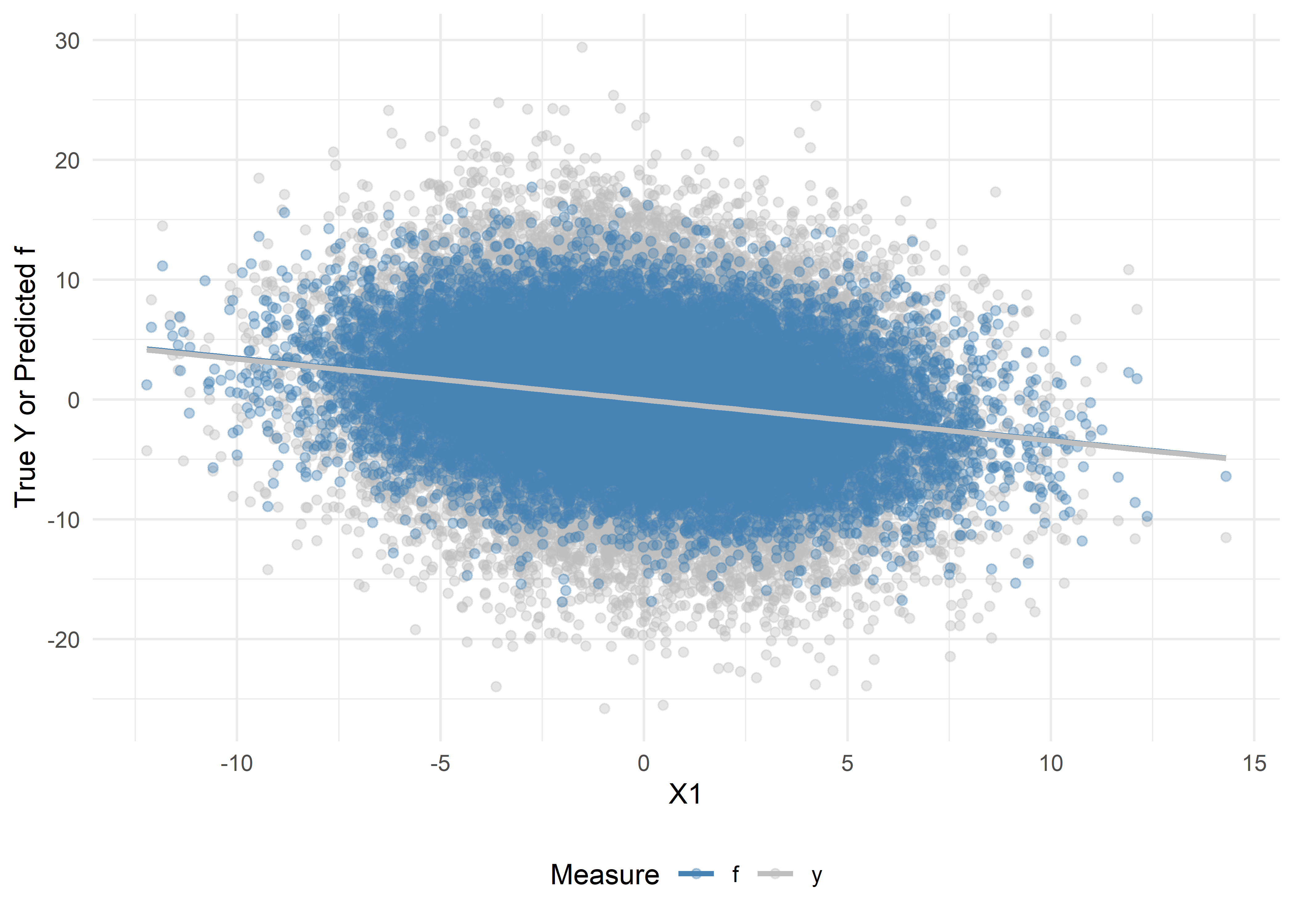

# Density plots
ggplot(dat_visualize, aes(x = Value, fill = Measure)) +
  theme_minimal() +
  geom_density(alpha = 0.4) +
  scale_fill_manual(values = c("steelblue", "gray")) +
  labs(
    x     = "Value",
    y     = "Density",
    fill  = "Measure"
  ) +
  theme(legend.position = "bottom")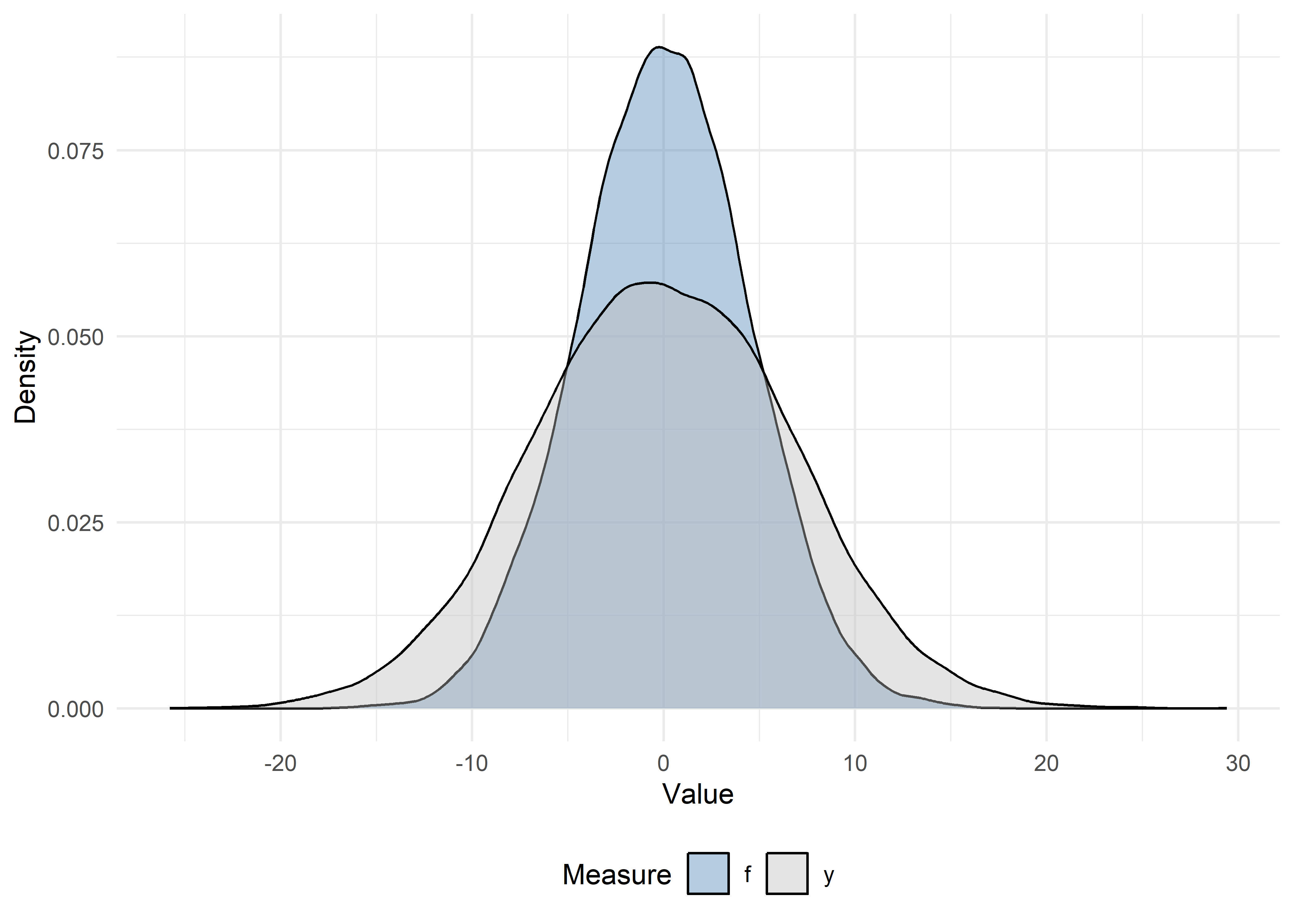

Notes

In the scatterplot, note that the predicted values \(f\) (in blue) are distributed similarly to the true \(Y\) (in gray).
In the density plot, you can see that the spread of \(f\) is slightly narrower than that of \(Y\).

Some Baselines: Oracle vs Naive vs Classical Inference

Before applying PB inference, let’s see what happens if we:

Regress the true Y on X1 for all observations (the oracle approach).
Regress the unlabeled predicted f on X1 (the naive approach).
Regress only the labeled true Y on X1 (the classical approach).

We will compare these to PB inference‐corrected estimates.

Exercise 3: Naive vs. Classical Model Fitting

Using the labeled and unlabeled sets, fit three models:

Oracle OLS on the full data using lm() with y ~ x1
Naive OLS on the unlabeled set using lm() with f ~ x1.
Classical OLS on the labeled set using lm() with y ~ x1.

Answer

# 1) Oracle: use the true outcomes for the full data (not possible in practice)
oracle_model <- lm(y ~ x1, data = dat_ipd)

# 2) Naive: treat f as if it were truth (only on unlabeled)
naive_model <- lm(f ~ x1, data = filter(dat_ipd, set_label == "unlabeled"))

# 3) Classical: regress true Y on X1, only on the labeled set
classical_model <- lm(y ~ x1, data = filter(dat_ipd, set_label == "labeled"))

Let’s also extract the coefficient summaries using the tidy method and compare the results of the three approaches:

Answer

oracle_df <- tidy(oracle_model) |>
  mutate(method = "Oracle") |>
  filter(term == "x1") |>
  select(method, estimate, std.error) 

naive_df <- tidy(naive_model) |>
  mutate(method = "Naive") |>
  filter(term == "x1") |>
  select(method, estimate, std.error) 

classical_df <- tidy(classical_model) |>
  mutate(method = "Classical") |>
  filter(term == "x1") |>
  select(method, estimate, std.error)

bind_rows(oracle_df, naive_df, classical_df)

# A tibble: 3 × 3
  method    estimate std.error
  <chr>        <dbl>     <dbl>
1 Oracle      -0.341   0.0132 
2 Naive       -0.340   0.00908
3 Classical   -0.356   0.0411

Notes

In this ideal setting, the naive coefficient is unbiased since the prediction model is correctly specified.
The classical coefficient is also unbiased but has a larger standard error due to the smaller sample size and additional random variation in the outcome.
The oracle provides the ideal baseline for these data.

PB Inference with `ipd::ipd()`

The single wrapper function ipd() implements multiple PB inference methods (e.g., Chen & Chen, PostPI, PPI, PPI++, PSPA) for various inferential tasks (e.g., mean and quantile estimation, ols, logistic, and Poisson regression).

Reminder

Basic usage of ipd():

ipd(
  formula = Y - f ~ X1,     # The downstream inferential model
  method  = "pspa",         # The PB inference method to run 
  model   = "ols",          # The type of inferential model
  data    = dat_ipd,        # A data.frame with columns:
                            #   - set_label: {"labeled", "unlabeled"}
                            #   - Y: true outcomes (for labeled data)
                            #   - f: predicted outcomes
                            #   - X covariates (here X1, X2, X3, X4)
  label   = "set_label"     # Column name indicating "labeled"/"unlabeled"
)

Exercise 4: PB Model Fitting via the Chen + Chen Estimator

Let’s run one method, chen, proposed by Gronsbell et al. (2026). The Chen + Chen estimator is a PB method that combines information from:

Labeled data (where the true outcome, \(Y\), and model predictions, \(f\), are available), and
Unlabeled data (where only model predictions, \(f\), are available).

Rather than treating the predicted outcomes with the same importance as the true outcomes, the method estimates a data-driven weight, \(\hat{\omega}\), and applies it to the predicted outcome contributions:

\[ \hat{\beta}_\text{cc} = \hat{\beta}_\text{classical} - \hat{\omega}\cdot (\hat{\gamma}_\text{naive}^l - \hat{\gamma}_\text{naive}^\text{all}), \]

where \(\hat{\beta}_{\rm classical}\) is the estimate from the classical regression, \(\hat{\gamma}_{\rm naive}^l\) is the estimate from the naive regression on the labeled data, \(\hat{\gamma}_{\rm naive}^\text{all}\) is the estimate from the naive regression on all the data, and \(\hat{\omega}\) reflects the amount of additional information carried by the predictions. By adaptively weighting the unlabeled information, the Chen + Chen estimator achieves greater precision than by using the labeled data alone, without sacrificing validity, even when the predictions are imperfect.

Let’s call the method using the ipd() function and collect the estimate for the slope of X1 in a linear regression (model = "ols"):

Answer

set.seed(123)

ipd_model <- ipd(
  formula = y - f ~ x1,
  data    = dat_ipd,
  label   = "set_label",
  method  = "chen",
  model   = "ols"
)

ipd_model

IPD inference summary
  Method:   chen 
  Model:    ols 
  Formula:  y - f ~ x1 

Coefficients:
             Estimate Std. Error  z value Pr(>|z|)    
(Intercept) -0.224224   0.104333  -2.1491  0.03162 *  
x1          -0.330246   0.032247 -10.2412  < 2e-16 ***
---
Signif. codes:  0 '***' 0.001 '**' 0.01 '*' 0.05 '.' 0.1 ' ' 1

The ipd_model is an S4 object with slots for things like the coefficient, se, ci, coefTable, fit, formula, data_l, data_u, method, model, and intercept. We can extract the coefficient table using ipd’s tidy helper and compare with the naive and classical methods:

Answer

# Extract the coefficient estimates
ipd_df <- tidy(ipd_model) |>
  mutate(method = "Chen + Chen") |>
  filter(term == "x1") |>
  select(method, estimate, std.error)

# Combine with oracle, naive, and classical:
compare_tab <- bind_rows(oracle_df, naive_df, classical_df, ipd_df)
compare_tab

# A tibble: 4 × 3
  method      estimate std.error
  <chr>          <dbl>     <dbl>
1 Oracle        -0.341   0.0132 
2 Naive         -0.340   0.00908
3 Classical     -0.356   0.0411 
4 Chen + Chen   -0.330   0.0322

Exercise 5: Visualizing Uncertainty

Let’s plot the coefficient estimates and 95% CIs for each of the naive, classical, and PB methods:

Answer

# Forest plot of estimates and 95% confidence intervals
compare_tab |>
  mutate(
    lower = estimate - 1.96 * std.error,
    upper = estimate + 1.96 * std.error
  ) |>
  ggplot(aes(x = estimate, y = method)) +
    geom_point(size = 2) +
    geom_errorbarh(aes(xmin = lower, xmax = upper), height = 0.2) +
    geom_vline(xintercept = b1[1], linetype = "dashed", color = "red") +
    labs(
      title = "Comparison of slope estimates \u00B1 1.96·SE",
      x = expression(hat(beta)[X1]),
      y = ""
    ) +
    theme_minimal()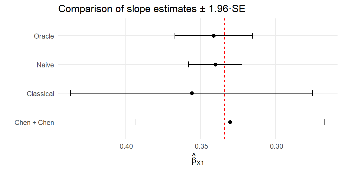

Notes

The dashed red line is the true data-generating effect for \(X_1\).
Here, all the methods are unbiased.
The classical approach has the widest interval, the naive interval is artificially too narrow, but Chen + Chen has intervals that are well calibrated.

Comparison of Results with Imperfect Predictions

Exercise 6: Imperfect Predictions

Now, let us repeat Exercises 1-5, but with \(X_1, \ldots, X_5\) omitted from the training of the prediction function:

predset_ind = 6 : 10

We will compare these results with the ideal case in the previous exercises. Here, since the predictions do not include \(X_1\), we should not be able to recover the true association between \(Y\) and \(X_1\).

Answer

Data Generation

set.seed(123)

dat_ipd2 <- simple_data_gen(
    n = n,               
    p = p,                
    prop_lab = 0.1,      
    total_var = 20,       
    ratio_var = 1,      
    rho = 0,             
    sigma_y = 1,          
    beta = c(b1, b2),    
    predset_ind = 6:10   # Omitting X1, ..., X5
)

Plotting the Data

# Prepare data
dat_visualize2 <- dat_ipd2 |> 
  select(x1, y, f) |>
  pivot_longer(y:f, names_to = "Measure", values_to = "Value") |>
  arrange(Measure)

# Scatter + trend lines
ggplot(dat_visualize2, aes(x = x1, y = Value, color = Measure)) +
  theme_minimal() +
  geom_point(alpha = 0.4) +
  geom_smooth(method = "lm", se = FALSE) +
  scale_color_manual(values = c("steelblue", "gray")) +
  labs(
    x     = "X1",
    y     = "True Y or Predicted f",
    color = "Measure"
  ) +
  theme(legend.position = "bottom")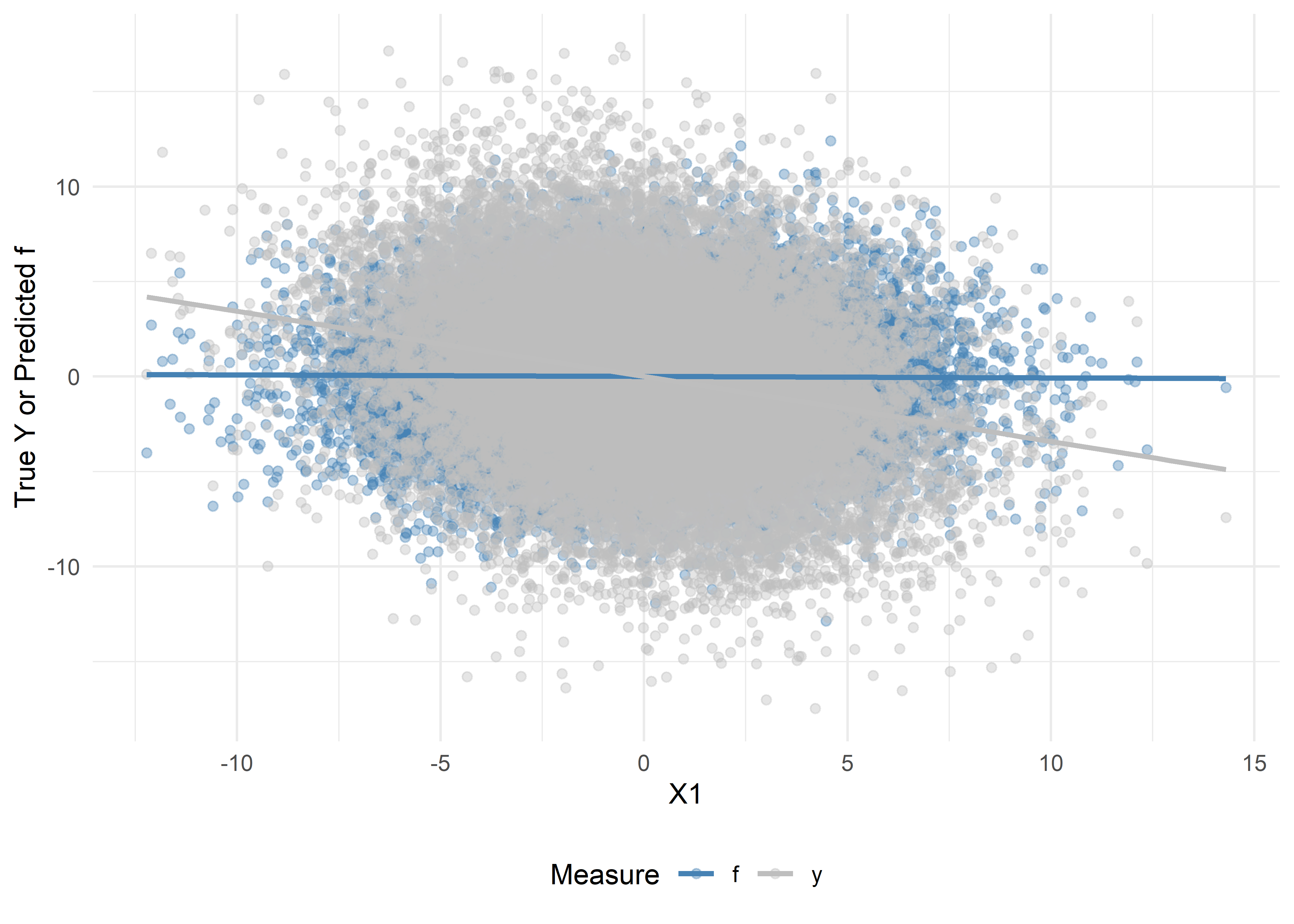

# Density plots
ggplot(dat_visualize2, aes(x = Value, fill = Measure)) +
  theme_minimal() +
  geom_density(alpha = 0.4) +
  scale_fill_manual(values = c("steelblue", "gray")) +
  labs(
    x     = "Value",
    y     = "Density",
    fill  = "Measure"
  ) +
  theme(legend.position = "bottom")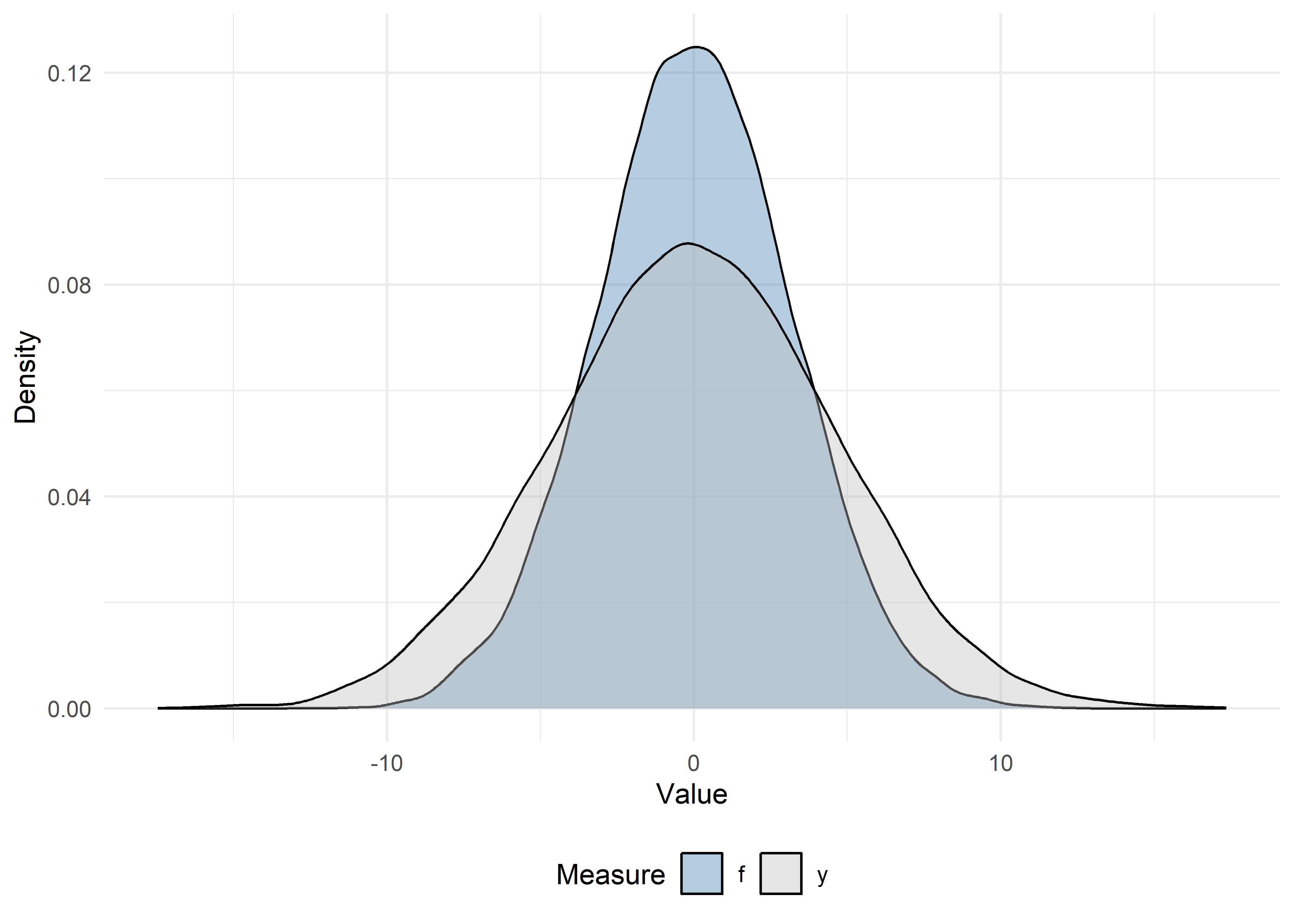

Oracle vs Naive vs Classical Inference

# 1) Oracle: use the true outcomes for the full data (not possible in practice)
oracle_model2 <- lm(y ~ x1, data = dat_ipd2)

# 2) Naive: treat f as if it were truth (only on unlabeled)
naive_model2 <- lm(f ~ x1, data = filter(dat_ipd2, set_label == "unlabeled"))

# 3) Classical: regress true Y on X1, only on the labeled set
classical_model2 <- lm(y ~ x1, data = filter(dat_ipd2, set_label == "labeled"))

oracle_df2 <- tidy(oracle_model2) |>
  mutate(method = "Oracle") |>
  filter(term == "x1") |>
  select(method, estimate, std.error) 

naive_df2 <- tidy(naive_model2) |>
  mutate(method = "Naive") |>
  filter(term == "x1") |>
  select(method, estimate, std.error) 

classical_df2 <- tidy(classical_model2) |>
  mutate(method = "Classical") |>
  filter(term == "x1") |>
  select(method, estimate, std.error)

bind_rows(oracle_df2, naive_df2, classical_df2)

# A tibble: 3 × 3
  method    estimate std.error
  <chr>        <dbl>     <dbl>
1 Oracle    -0.343     0.00882
2 Naive     -0.00775   0.00664
3 Classical -0.371     0.0272

PB Model Fitting via the Chen + Chen Estimator

set.seed(123)

ipd_model2 <- ipd(
  formula = y - f ~ x1,
  data    = dat_ipd2,
  label   = "set_label",
  method  = "chen",
  model   = "ols"
)

ipd_model2

IPD inference summary
  Method:   chen 
  Model:    ols 
  Formula:  y - f ~ x1 

Coefficients:
             Estimate Std. Error  z value Pr(>|z|)    
(Intercept)  0.096086   0.065442   1.4683    0.142    
x1          -0.370577   0.020917 -17.7163   <2e-16 ***
---
Signif. codes:  0 '***' 0.001 '**' 0.01 '*' 0.05 '.' 0.1 ' ' 1

# Extract the coefficient estimates
ipd_df2 <- tidy(ipd_model2) |>
  mutate(method = "Chen + Chen") |>
  filter(term == "x1") |>
  select(method, estimate, std.error)

# Combine with naive & classical:
compare_tab2 <- bind_rows(oracle_df2, naive_df2, classical_df2, ipd_df2)
compare_tab2

# A tibble: 4 × 3
  method      estimate std.error
  <chr>          <dbl>     <dbl>
1 Oracle      -0.343     0.00882
2 Naive       -0.00775   0.00664
3 Classical   -0.371     0.0272 
4 Chen + Chen -0.371     0.0209

Visualizing Uncertainty

# Forest plot of estimates and 95% confidence intervals
compare_tab2 |>
  mutate(
    lower = estimate - 1.96 * std.error,
    upper = estimate + 1.96 * std.error
  ) |>
  ggplot(aes(x = estimate, y = method)) +
    geom_point(size = 2) +
    geom_errorbarh(aes(xmin = lower, xmax = upper), height = 0.2) +
    geom_vline(xintercept = b1[1], linetype = "dashed", color = "red") +
    labs(
      title = "Comparison of slope estimates \u00B1 1.96·SE",
      x = expression(hat(beta)[X1]),
      y = ""
    ) +
    theme_minimal()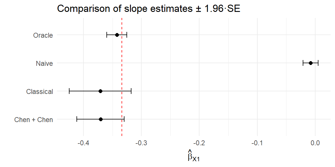

Notes

Plotting the Data

In the scatterplot, note that the predicted values \(f\) (in blue) lie more tightly along the fitted trend line than the true \(Y\) (in gray), indicating stronger correlation with \(X_1\).
In the density plot, you can see that the spread of \(f\) is narrower than that of \(Y\), illustrating that the predictive model has reduced variance.

Naive vs Classical Inference

The naive coefficient is attenuated, or biased toward zero, since the predictions are imperfect.
The classical coefficient is unbiased but has a larger standard error due to the smaller sample size.

PB Model Fitting va the Chen + Chen Estimator

The dashed red line is the true data-generating effect for \(X_1\).
Compare how far each method’s interval is from this line.
The naive approach severely underestimates both the effect estimate and its standard error, while Chen + Chen is unbiased and more efficient than the classical approach.
The efficiency gain is not as high compared to the perfect prediction scenario since the residual correlation between \(y\) and \(f\) is smaller

Exercise 7: Inspecting Results

Use tidy(), glance(), and augment() on ipd_model. Compare the coefficient estimate and standard error for X1 with the naive fit.

Answer

tidy(ipd_model)

# A tibble: 2 × 5
  term        estimate std.error conf.low conf.high
  <chr>          <dbl>     <dbl>    <dbl>     <dbl>
1 (Intercept)   -0.224    0.104    -0.429   -0.0197
2 x1            -0.330    0.0322   -0.393   -0.267

glance(ipd_model)

# A tibble: 1 × 6
  method model intercept nobs_labeled nobs_unlabeled call      
  <chr>  <chr> <lgl>            <int>          <int> <chr>     
1 chen   ols   TRUE              2551          22449 y - f ~ x1

augment(ipd_model) |> glimpse()

Rows: 22,449
Columns: 15
$ y         <dbl> 0.520872, -7.907675, -6.070025, 6.041134, -3.091775, 5.50057…
$ x1        <dbl> -3.7409669, 3.7360163, -3.2863856, 3.2313674, 3.7157033, 0.1…
$ x2        <dbl> 0.3358049, 3.8872286, -0.2270680, 0.9662234, 1.0364182, -2.6…
$ x3        <dbl> -3.7769611, 0.9883840, -4.4891339, 5.7711764, 0.6166084, 4.0…
$ x4        <dbl> 4.3382493, -4.2897707, 2.5735992, 2.2532995, -5.4164657, -4.…
$ x5        <dbl> -6.12151716, 1.01182690, -1.32007492, 1.62906763, -1.1307161…
$ x6        <dbl> -1.88428832, -2.32594242, 0.22120367, 3.69702327, -0.4563829…
$ x7        <dbl> -0.8790863, 0.1693632, 0.2598034, 1.8054718, 1.1521277, -0.1…
$ x8        <dbl> -5.64360288, -0.41344329, -1.16952884, -0.57129676, 1.196338…
$ x9        <dbl> 0.8406827, 2.6579939, -3.1565336, 4.9834037, 1.5231282, -1.4…
$ x10       <dbl> 3.8708865, 1.1378312, 1.2673506, 0.3500095, 5.6507155, 1.574…
$ f         <dbl> -2.0778359, -3.4210568, -1.4953638, 6.2205242, -3.4129538, 6…
$ set_label <chr> "unlabeled", "unlabeled", "unlabeled", "unlabeled", "unlabel…
$ .fitted   <dbl> 1.01121686, -1.45803011, 0.86109300, -1.29137161, -1.4513217…
$ .resid    <dbl> -0.4903448, -6.4496451, -6.9311184, 7.3325060, -1.6404531, 5…

# Compare with naive
broom::tidy(naive_model)

# A tibble: 2 × 5
  term        estimate std.error statistic   p.value
  <chr>          <dbl>     <dbl>     <dbl>     <dbl>
1 (Intercept)   0.0215   0.0288      0.745 4.56e-  1
2 x1           -0.340    0.00908   -37.4   1.06e-297

Summary and Key Takeaways

Naive regression on predicted outcomes can be biased and anti-conservative.
Classical regression on the labeled data alone is unbiased but inefficient when the labeled set is small.
PB methods strike a balance: they are unbiased, but potentially more efficient than the classical approach.
Even with ‘simple’ linear prediction models, PB corrections can improve inference on downstream regression coefficients.

Further Exploration

Try other methods such as PPI++ ("ppi_plusplus"). How do the results compare?
Repeat the analysis for a logistic model by setting model = "logistic" in both simdat() and ipd().

Simulating Data with `ipd::simdat()`

simdat() generates synthetic datasets for several inferential settings.

simdat(
  n,        # Numeric vector of length 3: c(n_train, n_labeled, n_unlabeled)
  effect,   # Numeric: true effect size for simulation
  sigma_Y,  # Numeric: residual standard deviation
  model,    # Character: one of "mean", "quantile", "ols", "logistic", "poisson"
  ...       # Additional arguments
)

This function returns a data.frame with columns:

X1, X2, ...: covariates
Y: true outcome (for training, labeled, and unlabeled subsets)
f: predictions from the model (for labeled and unlabeled subsets)
set_label: character indicating “training”, “labeled”, or “unlabeled”.

The ipd::simdat() function makes it easy to generate:

A training set (where you fit your prediction model),
A labeled set (where you observe the true \(Y\)),
An unlabeled set (where \(Y\) is presumed missing but you compute predictions \(f\)).

We supply the sample sizes, n = c(n_train, n_label, n_unlabel), an effect size (effect), residual standard deviation (sigma_Y; i.e., how much random noise is in the data), and a model type ("ols", "logistic", etc.). In this tutorial, we focus on a continuous outcome generated from a linear regression model ("ols"). We can also optionally shift and scale the predictions (via the shift and scale arguments) to control how the predicted outcomes relate to their true underlying counterparts.

Extra Activity: Generating Data with `simdat()`

Try generating data with the simdat() function. Let us generate a synthetic dataset for a linear model with:

5,000 training observations
500 labeled observations
1,500 unlabeled observations
Effect size = 1.5
Residual SD = 3
Predictions shifted by 1 and scaled by 2

Answer

set.seed(123)

# n_t = 5000, n_l = 500, n_u = 1500
n <- c(5000, 500, 1500)

# Effect size = 1.5, noise sd = 3, model = "ols" (ordinary least squares)
# We also shift the mean of the predictions by 1 and scale their values by 2
dat <- simdat(
  n       = n,
  effect  = 1.5,
  sigma_Y = 3,
  model   = "ols",
  shift   = 1,
  scale   = 2
)

# The resulting data.frame `dat` has columns:
#  - X1, X2, X3, X4: Four simulated covariates (all numeric ~ N(0,1))
#  - Y             : True outcome (available in unlabeled set for simulation)
#  - f             : Predicted outcome (Generated internally in simdat)
#  - set_label     : {"training", "labeled", "unlabeled"}

# Quick look:
dat |> 
  group_by(set_label) |> 
  summarize(n = n())

# A tibble: 3 × 2
  set_label     n
  <chr>     <int>
1 labeled     500
2 training   5000
3 unlabeled  1500

Let us also inspect the first few rows of each subset:

Answer

# Training set
dat |>
  filter(set_label == "training") |>
  glimpse()

Rows: 5,000
Columns: 7
$ X1        <dbl> -0.56047565, -0.23017749, 1.55870831, 0.07050839, 0.12928774…
$ X2        <dbl> -1.61803670, 0.37918115, 1.90225048, 0.60187427, 1.73234970,…
$ X3        <dbl> -0.91006117, 0.28066267, -1.03567040, 0.27304874, 0.53779815…
$ X4        <dbl> -1.119992047, -1.015819127, 1.258052722, -1.001231731, -0.40…
$ Y         <dbl> 3.8625325, -1.6575634, 4.1872914, -3.3624963, 6.9978916, 1.5…
$ f         <dbl> NA, NA, NA, NA, NA, NA, NA, NA, NA, NA, NA, NA, NA, NA, NA, …
$ set_label <chr> "training", "training", "training", "training", "training", …

# Labeled set
dat |>
  filter(set_label == "labeled") |>
  glimpse()

Rows: 500
Columns: 7
$ X1        <dbl> -0.4941739, 1.1275935, -1.1469495, 1.4810186, 0.9161912, 0.3…
$ X2        <dbl> -0.15062996, 0.80094056, -1.18671785, 0.43063636, 0.21674709…
$ X3        <dbl> 2.0279109, -1.4947497, -1.5729492, -0.3002123, -0.7643735, -…
$ X4        <dbl> 0.53495620, 0.36182362, -1.89096604, -1.40631763, -0.4019282…
$ Y         <dbl> 2.71822922, 1.72133689, 0.86081066, 3.77173123, -2.77191549,…
$ f         <dbl> 0.67556303, -0.13706321, -1.75579589, 0.84146158, 0.15512973…
$ set_label <chr> "labeled", "labeled", "labeled", "labeled", "labeled", "labe…

# Unlabeled set
dat |>
  filter(set_label == "unlabeled") |>
  glimpse()

Rows: 1,500
Columns: 7
$ X1        <dbl> -1.35723063, -1.29269781, -1.51720731, 0.85917603, -1.214617…
$ X2        <dbl> 0.01014789, 1.56213812, 0.41284605, -1.18886219, 0.71454993,…
$ X3        <dbl> -1.42521509, 1.73298966, 1.66085181, -0.85343610, 0.26905593…
$ X4        <dbl> -1.1645365, -0.2522693, -1.3945975, 0.3959429, 0.5980741, 1.…
$ Y         <dbl> -3.8296223, -3.0350282, -5.3736718, 2.6076634, -4.7813463, -…
$ f         <dbl> -1.9014253, -0.1679210, -0.3030749, 0.1249168, -0.8998546, -…
$ set_label <chr> "unlabeled", "unlabeled", "unlabeled", "unlabeled", "unlabel…

Notes

Rows where set_label == "training" form an internal training set. Here, Y is observed, but f is NA, as we learn the prediction rule in this set.
Rows where set_label == "labeled" also have both Y and f. In practice, f will be generated by your own prediction model; for simulation, simdat does so automatically.
Rows where set_label == "unlabeled" have Y for posterity (but in a real‐data scenario, you would not know Y); simdat still generates Y, but the PB routines will not use these. The column f always contains ‘predicted’ values.

Optional: Generating Your Own Predictions

In practice, we would take the training portion and fit an AI/ML model to predict \(Y\) from \((X_1, X_2, X_3, X_4)\). This is done automatically by the simdat function, but this optional activity gives you a hands-on implementation.

Extra Activity: Fitting a Linear Prediction Model

Fit a linear prediction model on the training data:

Answer

# 1) Subset training set
dat_train <- dat |> 
  filter(set_label == "training")

# 2) Fit a linear model: Y ~ X1 + X2 + X3 + X4
lm_pred <- lm(Y ~ X1 + X2 + X3 + X4, data = dat_train)

# 3) Prepare a full-length vector of NA
dat$f_pred <- NA_real_

# 4) Identify the rows to predict (all non-training rows)
idx_analytic <- dat$set_label != "training"

# 5) Generate predictions just once on that subset (shifted and scaled to match)
pred_vals <- (predict(lm_pred, newdata = dat[idx_analytic, ]) - 1) / 2

# 6) Insert them back into the full data frame
dat$f_pred[idx_analytic] <- pred_vals

# 7) Verify: `f_pred` is equal to `f` for the labeled and unlabeled data
dat |> 
  select(set_label, Y, f, f_pred) |> 
  filter(set_label != "training") |>
  glimpse()

Rows: 2,000
Columns: 4
$ set_label <chr> "labeled", "labeled", "labeled", "labeled", "labeled", "labe…
$ Y         <dbl> 2.71822922, 1.72133689, 0.86081066, 3.77173123, -2.77191549,…
$ f         <dbl> 0.67556303, -0.13706321, -1.75579589, 0.84146158, 0.15512973…
$ f_pred    <dbl> 0.67556303, -0.13706321, -1.75579589, 0.84146158, 0.15512973…

Notes

lm(Y ~ X1 + X2 + X3 + X4, data = dat_train) fits an ordinary least squares (OLS) regression on the training subset.
predict(lm_pred, newdata = .) generates a new f (stored as f_pred) for each row outside of the training set.
In real workflows, you might use random forests (ranger::ranger()), gradients (xgboost::xgboost()), or any other ML algorithm; PB methods only require that you supply a vector of predictions, f, in your data.

Happy coding! Feel free to modify and extend these exercises for your own data.

This is the end of the module. We hope this was informative! For question/concerns/suggestions, please reach out to ssalerno@fredhutch.org

Overview

Installation and Setup

Function References

ipd()

Supported Methods

Tidy Methods

Simulating Data

Exercise 1: Data Generation

Comparison of the True vs Predicted Outcomes

Exercise 2: Plotting the Data

Some Baselines: Oracle vs Naive vs Classical Inference

Exercise 3: Naive vs. Classical Model Fitting

PB Inference with ipd::ipd()

Exercise 4: PB Model Fitting via the Chen + Chen Estimator

Exercise 5: Visualizing Uncertainty

Comparison of Results with Imperfect Predictions

Exercise 6: Imperfect Predictions

Data Generation

Plotting the Data

Oracle vs Naive vs Classical Inference

PB Model Fitting via the Chen + Chen Estimator

Visualizing Uncertainty

Plotting the Data

Naive vs Classical Inference

PB Model Fitting va the Chen + Chen Estimator

Exercise 7: Inspecting Results

Summary and Key Takeaways

Further Exploration

Simulating Data with ipd::simdat()

Extra Activity: Generating Data with simdat()

Optional: Generating Your Own Predictions

Extra Activity: Fitting a Linear Prediction Model

`ipd()`

PB Inference with `ipd::ipd()`

Simulating Data with `ipd::simdat()`

Extra Activity: Generating Data with `simdat()`