Unit 00: Getting Started

Overview

Welcome to this workshop on Inference with Predicted Data (IPD)! In this module, we will:

Introduce the ipd package and its main functions.
Demonstrate how to generate synthetic data for different types of outcomes.
Fit and compare various IPD methods.
Inspect results using built-in tidy, glance, and augment methods.

Throughout the workshop, exercises are provided with solutions for practice.

Background and Motivation

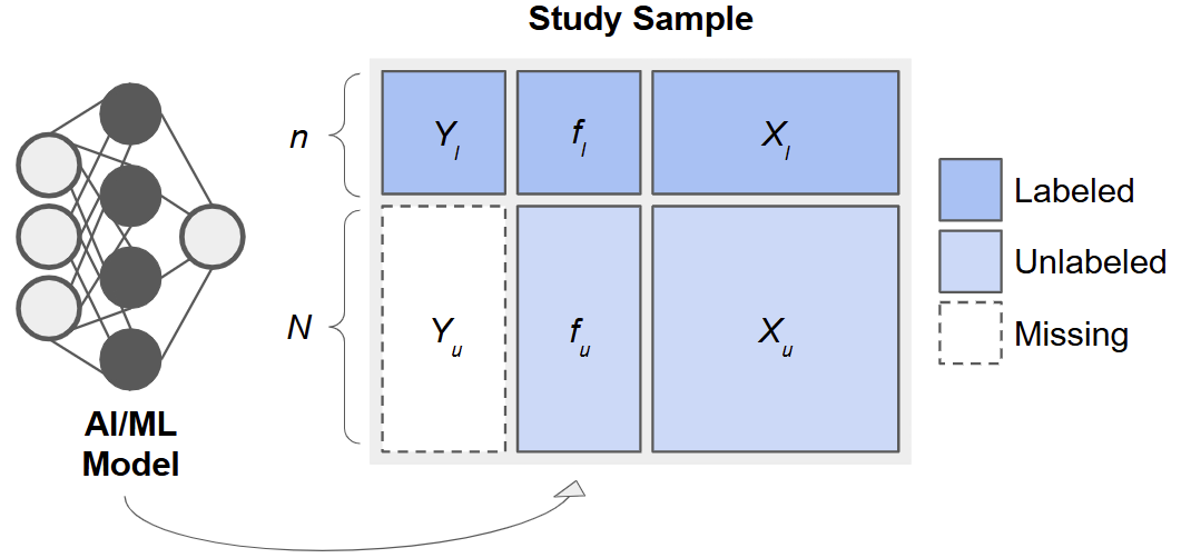
When an outcome, $Y$ , is costly or difficult to measure, it can be tempting to replace missing values with predictions, $f(\boldsymbol{X})$ , from a machine learning model (e.g., a random forest or neural network) built on easier-to-measure features, $\boldsymbol{X}$ . However, using $f$ as if it were the true outcome in downstream analyses, e.g., in estimating a regression coefficient, $\beta$ , for the association between $Y$ and $\boldsymbol{X}$ , leads to biased point estimates and underestimated uncertainty. Methods for Inference with Predicted Data (IPD) address this by leveraging a small subset of “labeled” data with true $Y$ values to calibrate inference in a larger “unlabeled” dataset.

The IPD Framework

Consider data arising from three sets of observations:

Training Set: $\{(X_j, Y_j)\}_{j=1}^{n_t}$ , used to fit a predictive model, $f(\cdot)$ .
Labeled Set: $\{(X_i, Y_i)\}_{i=1}^{n_l}$ , smaller sample with true outcomes measured.
Unlabeled Set: $\{(X_i)\}_{i=n_l +1}^{n_l + n_u}$ , only features available.

After fitting $f$ on the training set, we apply it to the labeled and unlabeled sets to obtain predictions $f_i = f(X_i)$ :

Overview of setup for common ‘inference with predicted data’ problems

Especially for ‘good’ predictions, it is tempting to treat $f_i$ as surrogate outcomes and use them to estimate quantities such as regression parameters, $\beta$ . However, as we will see, this leads to invalid inference. By combining the predicted $f_i$ with the observed $Y_i$ in the labeled set, we can calibrate our estimates and standard errors to achieve valid inference.

Key Formulas

Consider a simple linear regression model for the association between $Y$ and $X$ . We discuss the following potential estimators, which we will later implement using simulated data.

Naive Estimator

Using only the unlabeled predictions, the naive OLS estimator solves

$\hat\gamma_{\text{naive}} = \arg\min_\gamma \sum_{i\in U} (f_i - X_i'\gamma)^2.$

We are careful to write the coefficients for this model as $\gamma$ , because they bear no necessary correspondence with $\beta$ , except under the extremely restrictive scenario when $f$ perfectly captures the true regression function.

Classical Estimator

Instead, a valid approach would be to use only the labeled data. This classical estimator solves

$\hat\beta_{\text{classical}} = \arg\min_\beta \sum_{i\in L} (Y_i - X_i'\beta)^2.$ While this approach is valid, it has limited precision because $n_l$ is small in practice and we do not utilize any potential information from the (often much larger) unlabeled data.

IPD Estimators

Many estimators tailored to inference with predicted data share a similar form, as given in Ji et al. (2025):

$\widehat\beta_\text{ipd} = \arg\min_\beta \frac{1}{n_l}\sum_{i=1}^{n_l} \ell(X_i, Y_i) - \left[\frac{1}{n_l}\sum_{i=1}^{n_l} g(X_i, f_i) - \frac{1}{n_l+n_u}\sum_{i=n_l+1}^{n_l+n_u} g(X_i, f_i)\right],$

for some loss function, $\ell(\cdot)$ , such as the squared error loss for linear regression, and some $g(\cdot)$ , which they call the ‘imputed loss’. Here, the first term is exactly the classical estimator, which anchors these methods on a valid model, and the second term in the square brackets ‘augments’ the estimator with additional information from the predictions. This allows us to have an estimator that is provably unbiased and asymptotically at least as efficient as the classical estimator, which only uses a fraction of the data.

The Inference with Predicted Data (IPD) package implements several recent methods for IPD, such as Chen & Chen method of Gronsbell et al., the Prediction-Powered Inference (PPI) and PPI++ methods of Angelopoulos et al. (a) and Angelopoulos et al. (a), the Post-Prediction Inference (PostPI) method of Wang et al., and the Post-Prediction Adaptive Inference (PSPA) method of Miao et al. to conduct valid, efficient inference, even when a large proportion of outcomes are predicted.

In this first tutorial, we demonstrate how to:

Generate fully synthetic data with ipd::simdat().
Fit a simple linear prediction model (e.g., linear regression).
Apply ipd::ipd() to estimate the association, $\beta$ , between $Y$ and $X$ using labeled and unlabeled data.
Compare the naive, classical, and IPD estimates of $\beta$ .
Visualize these results.

Installation and Setup

First, insure you have the ipd package and some additional packages installed:

# Install these packages if you have not already:
# install.packages(c("ipd", "broom", "tidyverse", "patchwork"))

library(ipd)
library(broom)
library(tidyverse)
library(patchwork)

Throughout the workshop, we will use reproducible seeds and tidyverse conventions.

Function References

Below is a high-level summary of the core ipd functions.

`simdat()`

Generates synthetic datasets for various inferential models.

simdat(
  n,        # Numeric vector of length 3: c(n_train, n_labeled, n_unlabeled)
  effect,   # Numeric: true effect size for simulation
  sigma_Y,  # Numeric: residual standard deviation
  model,    # Character: one of "mean", "quantile", "ols", "logistic", "poisson"
  ...       # Additional arguments
)

This function returns a data.frame with columns:

X1, X2, ...: covariates
Y: true outcome (for training, labeled, and unlabeled subsets)
f: predictions from the model (for labeled and unlabeled subsets)
set_label: character indicating “training”, “labeled”, or “unlabeled”.

`ipd()`

Fits IPD methods for downstream inference on predicted data.

ipd(
  formula,      # A formula: e.g., Y - f ~ X1 + X2 + ...
  method,       # Character: one of "chen", "postpi_boot", "postpi_analytic", 
                # "ppi", "ppi_all", "ppi_plusplus", "pspa"
  model,        # Character: one of "mean", "quantile", "ols", "logistic", 
                # "poisson"
  data,         # Data frame containing columns for formula and label
  label,        # Character: name of the column with set labels ("labeled" and 
                # "unlabeled")
  ...           # Additional arguments
)

Supported Methods

chen: Chen and Chen estimator (Gronsbell et al., 2025)
postpi_analytic: analytic post-prediction inference (Wang et al., 2020).
postpi_boot: bootstrap post-prediction inference Wang et al., 2020).
ppi: prediction-powered inference (Angelopoulos et al., 2023)
ppi_plusplus: PPI++ (PPI with data-driven weighting; Angelopoulos et al., 2024)
ppi_a: PPI using all data (Gronsbell et al., 2025)
pspa: assumption-lean and data-adaptive post-prediction inference (Miao et al., 2024)

Tidy Methods

print() and summary(): display model summaries.
tidy(): return a tibble of estimates and standard errors.
glance(): return a one-row tibble of model-level metrics.
augment(): return the original data with fitted values and residuals.

Simulating Data

The ipd::simdat() function makes it easy to generate:

A training set (where you fit your prediction model),
A labeled set (where you observe the true $Y$ ),
An unlabeled set (where $Y$ is presumed missing but you compute predictions $f$ ).

We supply the sample sizes, n = c(n_train, n_label, n_unlabel), an effect size (effect), residual standard deviation (sigma_Y; i.e., how much random noise is in the data), and a model type ("ols", "logistic", etc.). In this tutorial, we focus on a continuous outcome generated from a linear regression model ("ols"). We can also optionally shift and scale the predictions (via the shift and scale arguments) to control how the predicted outcomes relate to their true underlying counterparts.

Exercise 1: Data Generation

Let us generate a synthetic dataset for a linear model with:

5,000 training observations
500 labeled observations
1,500 unlabeled observations
Effect size = 1.5
Residual SD = 3
Predictions shifted by 1 and scaled by 2

Note: Interactive exercises are provided below. Try writing your code in the first chunk; solutions are hidden in the second chunk.

set.seed(123)

# n_t = 5000, n_l = 500, n_u = 1500
n <- c(5000, 500, 1500)

# Effect size = 1.5, noise sd = 3, model = "ols" (ordinary least squares)
# We also shift the mean of the predictions by 1 and scale their values by 2
dat <- simdat(
  n       = n,
  effect  = 1.5,
  sigma_Y = 3,
  model   = "ols",
  shift   = 1,
  scale   = 2
)

# The resulting data.frame `dat` has columns:
#  - X1, X2, X3, X4: Four simulated covariates (all numeric ~ N(0,1))
#  - Y             : True outcome (available in unlabeled set for simulation)
#  - f             : Predicted outcome (Generated internally in simdat)
#  - set_label     : {"training", "labeled", "unlabeled"}

# Quick look:
dat |> 
  group_by(set_label) |> 
  summarize(n = n()) 
#> # A tibble: 3 × 2
#>   set_label     n
#>   <chr>     <int>
#> 1 labeled     500
#> 2 training   5000
#> 3 unlabeled  1500

Let us inspect the first few rows of each subset:

# Training set
dat |>
  filter(set_label == "training") |>
  glimpse()
#> Rows: 5,000
#> Columns: 7
#> $ X1        <dbl> -0.56047565, -0.23017749, 1.55870831, 0.07050839, 0.12928774…
#> $ X2        <dbl> -1.61803670, 0.37918115, 1.90225048, 0.60187427, 1.73234970,…
#> $ X3        <dbl> -0.91006117, 0.28066267, -1.03567040, 0.27304874, 0.53779815…
#> $ X4        <dbl> -1.119992047, -1.015819127, 1.258052722, -1.001231731, -0.40…
#> $ Y         <dbl> 3.8625325, -1.6575634, 4.1872914, -3.3624963, 6.9978916, 1.5…
#> $ f         <dbl> NA, NA, NA, NA, NA, NA, NA, NA, NA, NA, NA, NA, NA, NA, NA, …
#> $ set_label <chr> "training", "training", "training", "training", "training", …

# Labeled set
dat |>
  filter(set_label == "labeled") |>
  glimpse()
#> Rows: 500
#> Columns: 7
#> $ X1        <dbl> -0.4941739, 1.1275935, -1.1469495, 1.4810186, 0.9161912, 0.3…
#> $ X2        <dbl> -0.15062996, 0.80094056, -1.18671785, 0.43063636, 0.21674709…
#> $ X3        <dbl> 2.0279109, -1.4947497, -1.5729492, -0.3002123, -0.7643735, -…
#> $ X4        <dbl> 0.53495620, 0.36182362, -1.89096604, -1.40631763, -0.4019282…
#> $ Y         <dbl> 2.71822922, 1.72133689, 0.86081066, 3.77173123, -2.77191549,…
#> $ f         <dbl> 0.67556303, -0.13706321, -1.75579589, 0.84146158, 0.15512973…
#> $ set_label <chr> "labeled", "labeled", "labeled", "labeled", "labeled", "labe…

# Unlabeled set
dat |>
  filter(set_label == "unlabeled") |>
  glimpse()
#> Rows: 1,500
#> Columns: 7
#> $ X1        <dbl> -1.35723063, -1.29269781, -1.51720731, 0.85917603, -1.214617…
#> $ X2        <dbl> 0.01014789, 1.56213812, 0.41284605, -1.18886219, 0.71454993,…
#> $ X3        <dbl> -1.42521509, 1.73298966, 1.66085181, -0.85343610, 0.26905593…
#> $ X4        <dbl> -1.1645365, -0.2522693, -1.3945975, 0.3959429, 0.5980741, 1.…
#> $ Y         <dbl> -3.8296223, -3.0350282, -5.3736718, 2.6076634, -4.7813463, -…
#> $ f         <dbl> -1.9014253, -0.1679210, -0.3030749, 0.1249168, -0.8998546, -…
#> $ set_label <chr> "unlabeled", "unlabeled", "unlabeled", "unlabeled", "unlabel…

Explanation:

Rows where set_label == "training" form an internal training set. Here, Y is observed, but f is NA, as we learn the prediction rule in this set.

Rows where set_label == "labeled" also have both Y and f. In practice, f will be generated by your own prediction model; for simulation, simdat does so automatically.

Rows where set_label == "unlabeled" have Y for posterity (but in a real‐data scenario, you would not know Y); simdat still generates Y, but the IPD routines will not use these. The column f always contains ‘predicted’ values.

Fit a Linear Prediction Model

In practice, we would take the training portion and fit an AI/ML model to predict $Y$ from $(X_1, X_2, X_3, X_4)$ . This is done automatically by the simdat function, but for demonstration, let us fit a linear prediction model on the training data:

# 1) Subset training set
dat_train <- dat |> 
  filter(set_label == "training")

# 2) Fit a linear model: Y ~ X1 + X2 + X3 + X4
lm_pred <- lm(Y ~ X1 + X2 + X3 + X4, data = dat_train)

# 3) Prepare a full-length vector of NA
dat$f_pred <- NA_real_

# 4) Identify the rows to predict (all non–training rows)
idx_analytic <- dat$set_label != "training"

# 5) Generate predictions just once on that subset (shifted and scaled to match)
pred_vals <- (predict(lm_pred, newdata = dat[idx_analytic, ]) - 1) / 2 

# 6) Insert them back into the full data frame
dat$f_pred[idx_analytic] <- pred_vals

# 7) Verify: `f_pred` is equal to `f` for the labeled and unlabeled data
dat |> 
  select(set_label, Y, f, f_pred) |> 
  filter(set_label != "training") |>
  glimpse()
#> Rows: 2,000
#> Columns: 4
#> $ set_label <chr> "labeled", "labeled", "labeled", "labeled", "labeled", "labe…
#> $ Y         <dbl> 2.71822922, 1.72133689, 0.86081066, 3.77173123, -2.77191549,…
#> $ f         <dbl> 0.67556303, -0.13706321, -1.75579589, 0.84146158, 0.15512973…
#> $ f_pred    <dbl> 0.67556303, -0.13706321, -1.75579589, 0.84146158, 0.15512973…

Explanation of arguments:

lm(Y ~ X1 + X2 + X3 + X4, data = dat_train) fits an ordinary least squares (OLS) regression on the training subset.

predict(lm_pred, newdata = .) generates a new f (stored as f_pred) for each row outside of the training set.

Note: In real workflows, you might use random forests (ranger::ranger()), gradients (xgboost::xgboost()), or any other ML algorithm; the IPD methods only require that you supply a vector of predictions, f, in your data.

Create ‘Labeled’ and ‘Unlabeled’ datasets

We now split the data into two subsets:

labeled: those rows where we retain the true Y (to be used for final inference alongside their predictions).
unlabeled: those rows where we hide the true Y (we pretend we do not observe them; ipd will still require the f + covariates).

dat_ipd <- dat |>
  filter(set_label != "training") |>
  # Keep only the columns needed for downstream IPD
  select(set_label, Y, f, X1, X2, X3, X4) 

# Show counts:
dat_ipd |> 
  group_by(set_label) |> 
  summarize(n = n())
#> # A tibble: 2 × 2
#>   set_label     n
#>   <chr>     <int>
#> 1 labeled     500
#> 2 unlabeled  1500

Explanation:

After this step, dat_ipd has two groups:

labeled (500 rows where we observe both Y and f),

unlabeled (1500 rows where we only ‘observe’ f).

Comparison of the True vs Predicted Outcomes

Before modeling, it is helpful to see graphically how the predicted values, $f$ , compare to the true outcomes, $Y$ . We can visually assess the bias and variance of our predicted outcomes, $f$ , versus the true outcomes, $Y$ , in our analytic data by plotting:

Scatterplot of $Y$ and $f$ vs. $X_1$
Density plots of $Y$ and $f$

# Prepare data
dat_visualize <- dat_ipd |> 
  select(X1, Y, f) |>
  pivot_longer(Y:f, names_to = "Measure", values_to = "Value") |>
  arrange(Measure)

# Scatter + trend lines
ggplot(dat_visualize, aes(x = X1, y = Value, color = Measure)) +
  theme_minimal() +
  geom_point(alpha = 0.4) +
  geom_smooth(method = "lm", se = FALSE) +
  scale_color_manual(values = c("steelblue", "gray")) +
  labs(
    x     = "X1",
    y     = "True Y or Predicted f",
    color = "Measure"
  ) +
  theme(legend.position = "bottom")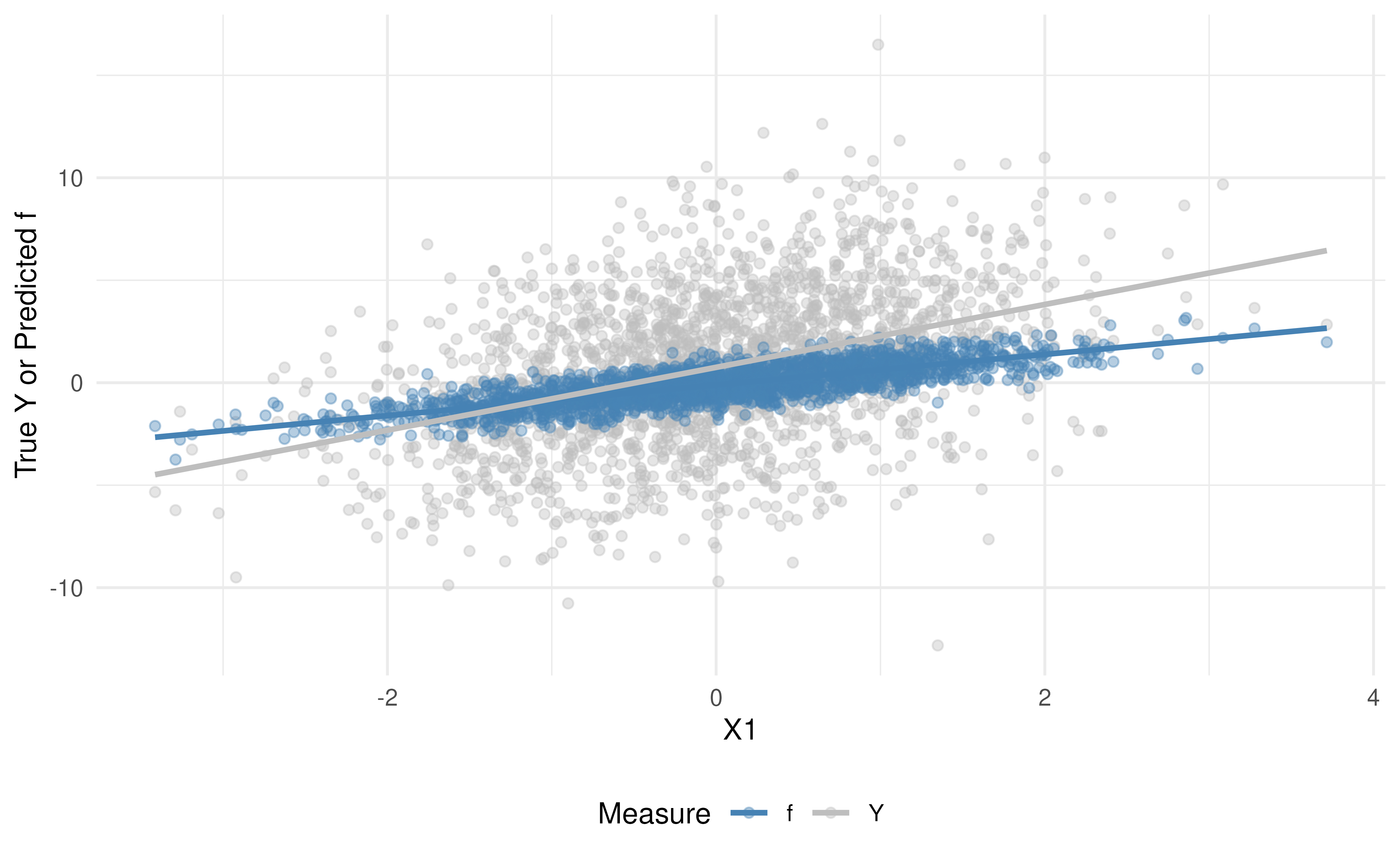

# Density plots
ggplot(dat_visualize, aes(x = Value, fill = Measure)) +
  theme_minimal() +
  geom_density(alpha = 0.4) +
  scale_fill_manual(values = c("steelblue", "gray")) +
  labs(
    x     = "Value",
    y     = "Density",
    fill  = "Measure"
  ) +
  theme(legend.position = "bottom")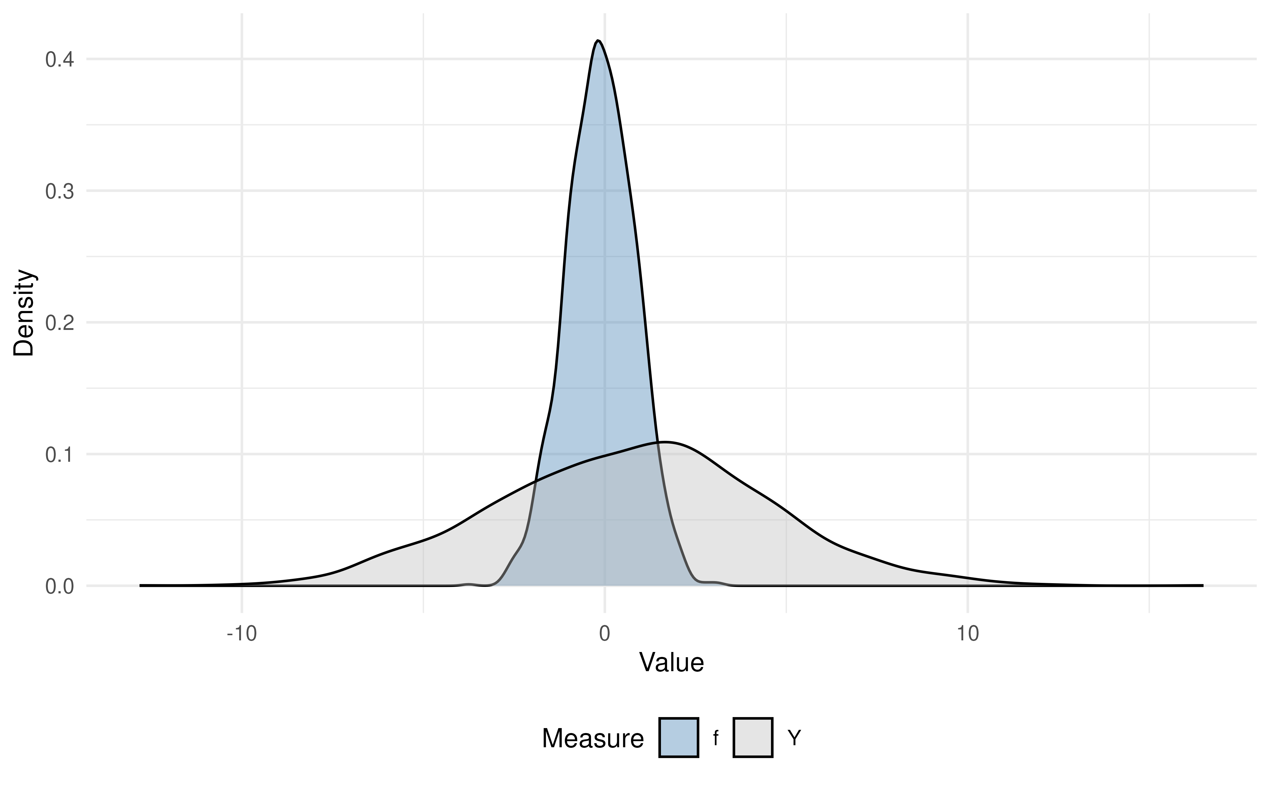

Interpretation:

In the scatterplot, note that the predicted values $f$ (in blue) lie more tightly along the fitted trend line than the true $Y$ (in gray), indicating stronger correlation with $X_1$ .

In the density plot, you can see that the spread of $f$ is narrower than that of $Y$ , illustrating that the predictive model has reduced variance (often due to “regression to the mean”).

Some Baselines: Naive vs Classical Inference

Before applying IPD, let’s see what happens if we:

Regress the unlabeled predicted f on X1 (the naive approach).
Regress only the labeled true Y on X1 (the classical approach).

We will compare these to IPD‐corrected estimates.

Exercise 2: Naive vs. Classical Model Fitting

Using the labeled and unlabeled sets, fit two models:

Naive OLS on the unlabeled set using lm() with f ~ X1.
Classical OLS on the labeled set using lm() with Y ~ X1.

# 1) Naive: treat f as if it were truth (only on unlabeled)
naive_model <- lm(f ~ X1, data = filter(dat_ipd, set_label == "unlabeled"))

# 2) Classical: regress true Y on X1, only on the labeled set
classical_model <- lm(Y ~ X1, data = filter(dat_ipd, set_label == "labeled"))

Let’s also extract the coefficient summaries using tidy and compare the results of the two approaches:

naive_df <- tidy(naive_model) |>
  mutate(method = "Naive") |>
  filter(term == "X1") |>
  select(method, estimate, std.error) 

classical_df <- tidy(classical_model) |>
  mutate(method = "Classical") |>
  filter(term == "X1") |>
  select(method, estimate, std.error)

bind_rows(naive_df, classical_df)
#> # A tibble: 2 × 3
#>   method    estimate std.error
#>   <chr>        <dbl>     <dbl>
#> 1 Naive        0.730    0.0145
#> 2 Classical    1.48     0.155

Expected behavior (interpretation):

The naive coefficient is attenuated, or biased toward zero, since the predictions are imperfect.

The classical coefficient is unbiased but has a larger standard error due to the smaller sample size.

IPD: Corrected Inference with `ipd::ipd()`

The single wrapper function ipd() implements multiple IPD methods (e.g., Chen & Chen, PostPI, PPI, PPI++, PSPA) for various inferential tasks (e.g., mean and quantile estimation, ols, logistic, and poisson regression).

Reminder: Basic usage of ipd():

ipd(
  formula = Y - f ~ X1,     # The downstream inferential model
  method  = "pspa"          # The IPD method to run 
  model   = "ols"           # The type of inferential model
  data    = dat_ipd,        # A data.frame with columns:
                            #   - set_label: {"labeled", "unlabeled"}
                            #   - Y: true outcomes (for labeled data)
                            #   - f: predicted outcomes
                            #   - X covariates (here X1, X2, X3, X4)
  label   = "set_label",    # Column name indicating "labeled"/"unlabeled"
)

Exercise 3: IPD Model Fitting via the PSPA Estimator

Let’s run one method, pspa, proposed by Miao et al., 2024. The PSPA estimator is an IPD method that combines information from:

Labeled data (where the true outcome, $Y$ , and model predictions, $f$ , are available), and
Unlabeled data (where only model predictions, $f$ , are available).

Rather than treating the predicted outcomes with importance as the true outcomes, the method estimates a data-driven weight, $\hat{\omega}$ , and applies it to the predicted outcome contributions:

$\hat{\beta}_\text{pspa} = \hat{\beta}_\text{classical} - \hat{\omega}\cdot (\hat{\gamma}_\text{naive}^l - \hat{\gamma}_\text{naive}^u),$

where $\hat{\beta}_{\rm classical}$ is the estimate from the classical regression, $\hat{\gamma}_{\rm naive}^l$ is the estimate from the naive regression in the labeled data, $\hat{\gamma}_{\rm naive}^u$ is the estimate from the naive regression in the unlabeled data, and $\hat{\omega}$ reflects the amount of additional information carried by the predictions. By adaptively weighting the unlabeled information, the PSPA estimator achieves greater precision than by using the labeled data alone, without sacrificing validity, even when the predictions are imperfect.

Let’s call the method using the ipd() function and collect the estimate for the slope of X1 in a linear regression (model = "ols"):

set.seed(123)
ipd_model <- ipd(
  formula = Y - f ~ X1,
  data    = dat_ipd,
  label   = "set_label",
  method  = "pspa",
  model   = "ols"
)

ipd_model
#> 
#> Call:
#>  Y - f ~ X1 
#> 
#> Coefficients:
#> (Intercept)          X1 
#>   0.8801364   1.4324759

The ipd_model is an S4 object with slots for things like the coefficient, se, ci, coefTable, fit, formula, data_l, data_u, method, model, and intercept. We can extract the coefficient table using ipd’s tidy helper and compare with the naive and classical methods:

# Extract the coefficient estimates
ipd_df <- tidy(ipd_model) |>
  mutate(method = "IPD") |>
  filter(term == "X1") |>
  select(method, estimate, std.error)

# Combine with naive & classical:
compare_tab <- bind_rows(naive_df, classical_df, ipd_df)
compare_tab
#> # A tibble: 3 × 3
#>   method    estimate std.error
#> * <chr>        <dbl>     <dbl>
#> 1 Naive        0.730    0.0145
#> 2 Classical    1.48     0.155 
#> 3 IPD          1.43     0.146

Exercise 4: Visualizing Uncertainty

Let’s plot the coefficient estimates and 95% CIs for each of the naive, classical, and IPD methods:

# Forest plot of estimates and 95% confidence intervals
compare_tab |>
  mutate(
    lower = estimate - 1.96 * std.error,
    upper = estimate + 1.96 * std.error
  ) |>
  ggplot(aes(x = estimate, y = method)) +
    geom_point(size = 2) +
    geom_errorbarh(aes(xmin = lower, xmax = upper), height = 0.2) +
    geom_vline(xintercept = 1.5, linetype = "dashed", color = "red") +
    labs(
      title = "Comparison of slope estimates \u00B1 1.96·SE",
      x = expression(hat(beta)[X1]),
      y = ""
    ) +
    theme_minimal()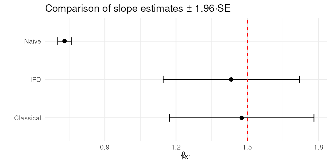

Interpretation:

The dashed red line at 1.5 is the true data-generating effect for $X_1$ .

Compare how far each method’s interval is from 1.5, and whether 1.5 lies inside each interval.

‘Naive’ often severely underestimates (biased); ‘Classical’ is unbiased but wide; IPD methods cluster around 1.5 with better coverage than ‘naive,’ often similar to classical but sometimes narrower.

Exercise 5: Inspecting Results

Use tidy(), glance(), and augment() on ipd_model. Compare the coefficient estimate and standard error for X1 with the naive fit.

tidy(ipd_model)
#>                    term  estimate std.error  conf.low conf.high
#> (Intercept) (Intercept) 0.8801364 0.1470190 0.5919845  1.168288
#> X1                   X1 1.4324759 0.1462767 1.1457788  1.719173
glance(ipd_model)
#>   method model include_intercept nobs_labeled nobs_unlabeled       call
#> 1   pspa   ols              TRUE          500           1500 Y - f ~ X1
augment(ipd_model) |> glimpse()
#> Rows: 1,500
#> Columns: 9
#> $ set_label <chr> "unlabeled", "unlabeled", "unlabeled", "unlabeled", "unlabel…
#> $ Y         <dbl> -3.8296223, -3.0350282, -5.3736718, 2.6076634, -4.7813463, -…
#> $ f         <dbl> -1.9014253, -0.1679210, -0.3030749, 0.1249168, -0.8998546, -…
#> $ X1        <dbl> -1.35723063, -1.29269781, -1.51720731, 0.85917603, -1.214617…
#> $ X2        <dbl> 0.01014789, 1.56213812, 0.41284605, -1.18886219, 0.71454993,…
#> $ X3        <dbl> -1.42521509, 1.73298966, 1.66085181, -0.85343610, 0.26905593…
#> $ X4        <dbl> -1.1645365, -0.2522693, -1.3945975, 0.3959429, 0.5980741, 1.…
#> $ .fitted   <dbl[,1]> <matrix[26 x 1]>
#> $ .resid    <dbl[,1]> <matrix[26 x 1]>

# Compare with naive
broom::tidy(naive_model)
#> # A tibble: 2 × 5
#>   term        estimate std.error statistic  p.value
#>   <chr>          <dbl>     <dbl>     <dbl>    <dbl>
#> 1 (Intercept)   -0.118    0.0146     -8.07 1.40e-15
#> 2 X1             0.730    0.0145     50.3  0

Summary and Key Takeaways

Naive regression on predicted outcomes is biased (point estimates are pulled toward zero and SEs are artificially small).
Classical regression on the labeled data alone is unbiased but inefficient when the labeled set is small.
IPD methods (Chen & Chen, PPI, PPI++, PostPI, PSPA) strike a balance: they use predictions to effectively enlarge sample size but adjust for prediction error to avoid bias.
Even with ‘simple’ linear prediction models, IPD corrections can drastically improve inference on downstream regression coefficients.

Further Exploration

Try other methods such as PPI++ ("ppi_plusplus"). How do the results compare?
Repeat the analysis for a logistic model by setting model = "logistic" in both simdat() and ipd().

Happy coding! Feel free to modify and extend these exercises for your own data.

References

Salerno, Stephen, et al. “ipd: An R Package for Conducting Inference on Predicted Data.” Bioinformatics (2025): btaf055.

This is the end of the module. We hope this was informative! For question/concerns/suggestions, please reach out to ssalerno@fredhutch.org

Stephen Salerno

June 24, 2025

Overview

Background and Motivation

The IPD Framework

Key Formulas

Naive Estimator

Classical Estimator

IPD Estimators

Installation and Setup

Function References

`simdat()`

`ipd()`

Supported Methods

Tidy Methods

Simulating Data

Exercise 1: Data Generation

Fit a Linear Prediction Model

Create ‘Labeled’ and ‘Unlabeled’ datasets

Comparison of the True vs Predicted Outcomes

Some Baselines: Naive vs Classical Inference

Exercise 2: Naive vs. Classical Model Fitting

IPD: Corrected Inference with `ipd::ipd()`

Exercise 3: IPD Model Fitting via the PSPA Estimator

Exercise 4: Visualizing Uncertainty

Exercise 5: Inspecting Results

Summary and Key Takeaways

Further Exploration

References

Unit 00: Getting Started

Stephen Salerno

June 24, 2025

Overview

Background and Motivation

The IPD Framework

Key Formulas

Naive Estimator

Classical Estimator

IPD Estimators

Installation and Setup

Function References

simdat()

ipd()

Supported Methods

Tidy Methods

Simulating Data

Exercise 1: Data Generation

Fit a Linear Prediction Model

Create ‘Labeled’ and ‘Unlabeled’ datasets

Comparison of the True vs Predicted Outcomes

Some Baselines: Naive vs Classical Inference

Exercise 2: Naive vs. Classical Model Fitting

IPD: Corrected Inference with ipd::ipd()

Exercise 3: IPD Model Fitting via the PSPA Estimator

Exercise 4: Visualizing Uncertainty

Exercise 5: Inspecting Results

Summary and Key Takeaways

Further Exploration

References

`simdat()`

`ipd()`

IPD: Corrected Inference with `ipd::ipd()`