Unit 03: BCR-ABL Fusion in B-Cell Leukemia

Background & Motivation

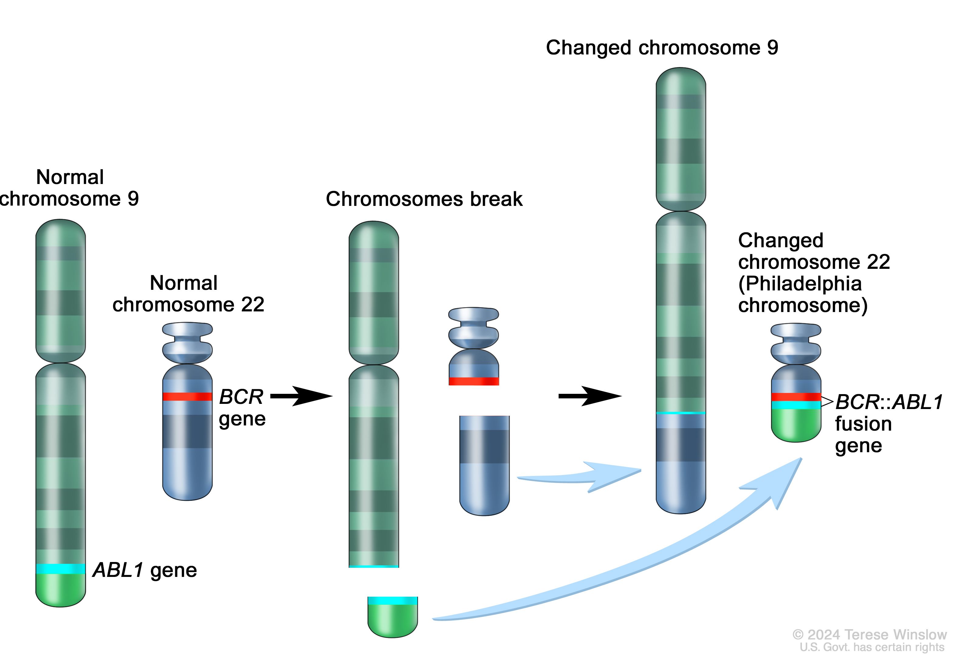
Acute lymphoblastic leukemia (ALL) is the most common childhood cancer, but it exhibits marked genetic heterogeneity, with distinct chromosomal translocations defining molecular subtypes with divergent prognoses and therapeutic responses. In B-cell lineage ALL, the BCR-ABL1 fusion (“breakpoint cluster region”/“Abelson”, i.e., the “Philadelphia chromosome”) arises from a t(9;22) translocation and encodes a constitutively active tyrosine kinase. This fusion was historically associated with poor outcomes, until the advent of targeted therapies (e.g., imatinib) revolutionized treatment and survival.

Source: https://www.cancer.gov/publications/dictionaries/cancer-terms/def/philadelphia-chromosome

High-density microarray profiling measures expression of over 7,000 genes in leukemic blast cells, enabling a form of “molecular diagnostics” where supervised learning can:

Classify fusion status or other genetic subtypes when cytogenetic assays (PCR, FISH) are unavailable.
Discover novel marker genes and pathways dysregulated by specific fusions.
Predict therapeutic response and stratify risk using expression-derived scores.

However, in many retrospective or multi-center cohorts, only a subset of patients undergo gold-standard fusion testing (e.g., RT-PCR for BCR-ABL1), leaving the majority “unlabeled.” A common workaround is to train a gene expression classifier on the small labeled subset and apply it to the larger unlabeled cohort. Yet, naive downstream analyses, treating predicted labels as ground truth, can yield biased effect estimates and understate uncertainty.

Inference with Predicted Data (IPD) offers a principled remedy: it combines a small labeled set with the predicted labels (e.g., with true fusion status) with a larger unlabeled set, adjusting both bias and variance. In this module, we will:

Describe the ALL and Golub Bioconductor datasets.
Subset the ALL data to B-cell ALL and filter to the top 500 variable probes.
Harmonize probes across platforms via gene symbols.
Split the ALL data and train three classifiers for BCR-ABL1 fusion status.
Predict on the holdout ALL and Golub B-cell ALL data using the ALL-trained classifier.
Apply IPD to estimate the association between fusion status and patient sex assigned at birth.

By the end, you will understand how to leverage expression-based predictions while maintaining valid inference on genetic subtypes in cohorts with partially missing gold-standard labels.

Note: For the data loading and prediction workflows, we will directly follow the Bioconductor MLInterfaces vignette by VJ Carey and P Atieno:

https://www.bioconductor.org/packages/devel/bioc/vignettes/MLInterfaces/inst/doc/MLprac2_2.html

Datasets Overview

We work with two public Bioconductor datasets:

ALL (ALL package): 128 samples of acute lymphoblastic leukemia (both B- and T-cell), profiled on the Affymetrix HGU95Av2 microarray. Phenotype data include BT (immunophenotype), mol.biol (molecular subtype including BCR-ABL1 or NEG), age, and sex.
Golub_Merge (golubEsets package): 72 samples of leukemias (ALL vs. AML), profiled on Affymetrix HGU6800. Phenotype data include ALL.AML, T.B.cell (lineage), age, and sex.

We will train our classifiers on a subset of the ALL data, test the model on the holdout ALL data, and perform IPD on the holdout ALL and Golub data.

Phenotype Reduction and Feature Filtering

We first narrow to B-cell ALL samples and reduce dimensionality by keeping the 500 most variable probes.

# Load the ALL data
data(ALL)

# Subset ALL to B-cell lineage (BT codes starting with "B")
bALL <- ALL[, substr(pData(ALL)$BT, 1, 1) == "B"]

# Keep only fusion-negative ("NEG") and fusion-positive ("BCR/ABL") samples
fus <- bALL[, bALL$mol.biol %in% c("NEG", "BCR/ABL")]

# Convert to factor with clear levels: NEG=0, BCR/ABL=1
fus$mol.biol <- factor(fus$mol.biol, levels = c("NEG", "BCR/ABL"))

# Compute median absolute deviation (MAD) for each probe
devs <- apply(exprs(fus), 1, mad)

# Select top 500 most variable probes by MAD ranking
top500 <- order(devs, decreasing = TRUE)[1:500]

# Subset ExpressionSet to top 500 probes
dat_filt <- fus[top500, ]

# Confirm dimensions: 500 probes x n samples
dim(exprs(dat_filt))
#> [1] 500  79

Explanation:

mad() is robust to outliers and captures variability.

Filtering saves time on downstream analysis without losing key signals.

We now have dat_filt, a filtered ALL dataset focused on B-cell lineage and the most informative probes.

Cross-Platform Probe Harmonization

To predict on the Golub data, which uses a different array, we map probes from each platform to gene symbols, then intersect to find a common gene set.

# Load the Golub data
data(Golub_Merge)

# Map HGU95Av2 probes (ALL) to gene symbols
gmap_all <- AnnotationDbi::select(
  hgu95av2.db,
  keys    = featureNames(dat_filt),
  columns = c("PROBEID","SYMBOL"),
  keytype = "PROBEID"
)

# HGU6800 probes (Golub) to gene symbols
gmap_golub <- AnnotationDbi::select(
  hu6800.db,
  keys    = featureNames(Golub_Merge),
  columns = c("PROBEID","SYMBOL"),
  keytype = "PROBEID"
)

# Identify common symbols
common_sym <- intersect(gmap_all$SYMBOL, gmap_golub$SYMBOL)

# For each symbol, pick the first associated probe
probe_all <- gmap_all |> 
  filter(SYMBOL %in% common_sym) |> 
  group_by(SYMBOL) |> 
  dplyr::slice(1) |> 
  drop_na()

probe_golub <- gmap_golub |> 
  filter(SYMBOL %in% common_sym) |> 
  group_by(SYMBOL) |> 
  dplyr::slice(1) |> 
  drop_na()

# Subset ExpressionSets to these probes
dat_train  <- dat_filt[probe_all$PROBEID, ]
eset_golub <- Golub_Merge[probe_golub$PROBEID, ]

# Further subset Golub to B-cell ALL samples
golub_bALL <- eset_golub[, pData(eset_golub)$T.B.cell == "B-cell" &
                           pData(eset_golub)$ALL.AML  == "ALL"]

featureNames(dat_train) <- probe_all$SYMBOL
rownames(exprs(dat_train)) <- probe_all$SYMBOL

featureNames(golub_bALL) <- probe_golub$SYMBOL
rownames(exprs(golub_bALL)) <- probe_golub$SYMBOL


# Confirm feature dimensions
dim(dat_train)    # features x ALL samples
#> Features  Samples 
#>      354       79
dim(golub_bALL)   # features x Golub B-cell ALL samples
#> Features  Samples 
#>      354       38

dat_train and golub_BALL now share the same gene-symbol feature set, ready for model training and transfer.

Exploratory Data Analysis

With our filtered training set (dat_train), we explore patterns using a heatmap and principal component analysis (PCA).

# Set subtype colors for visualization
fcol <- ifelse(dat_train$mol.biol == "NEG", "gray", "steelblue")

heatmap(exprs(dat_train), ColSideColors = fcol)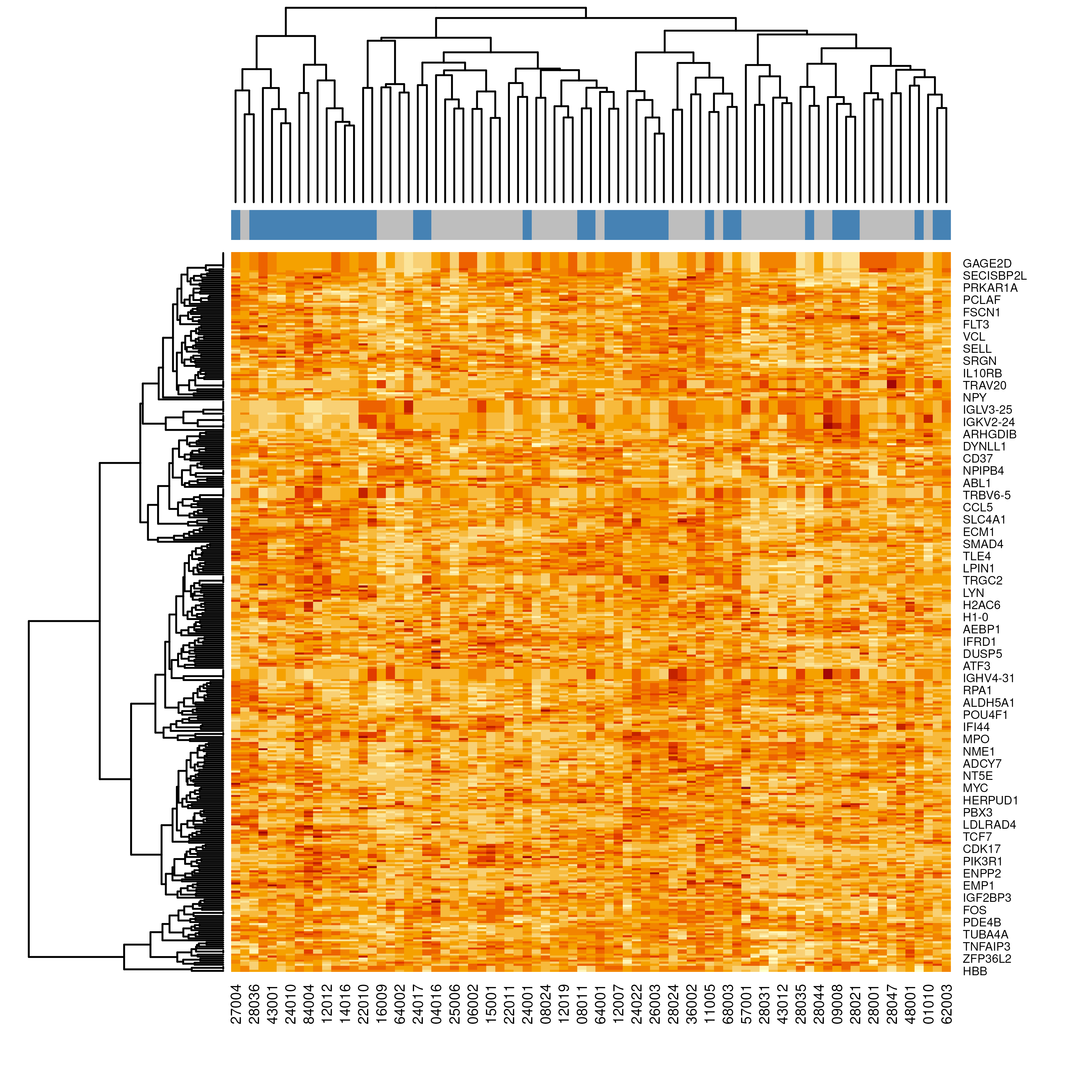

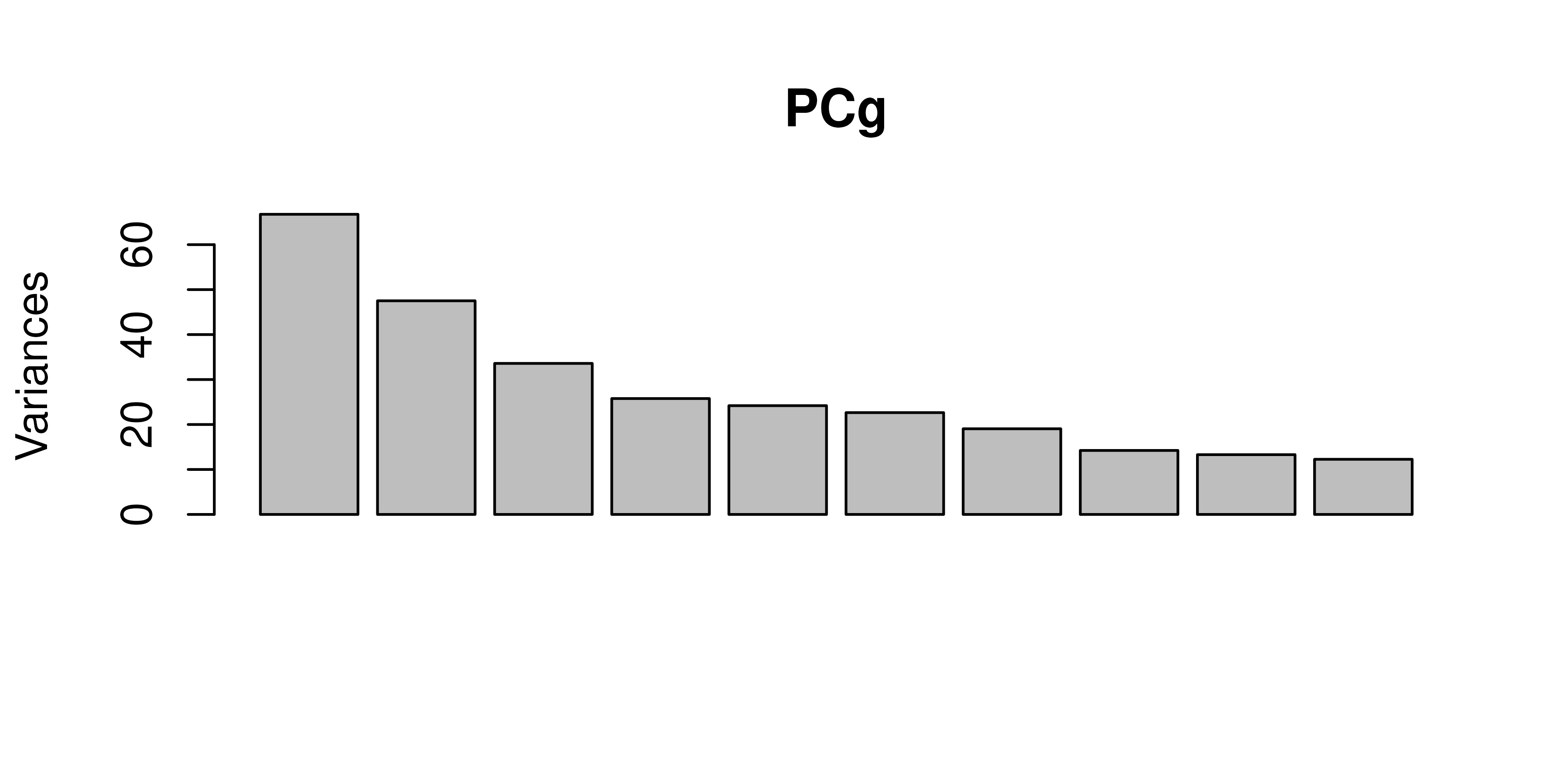
# PCA on samples
PCg <- prcomp(t(exprs(dat_train)))

# Scree plot
plot(PCg)

# Scatterplots of PCs
pairs(PCg$x[, 1:5], col = fcol, pch = 19)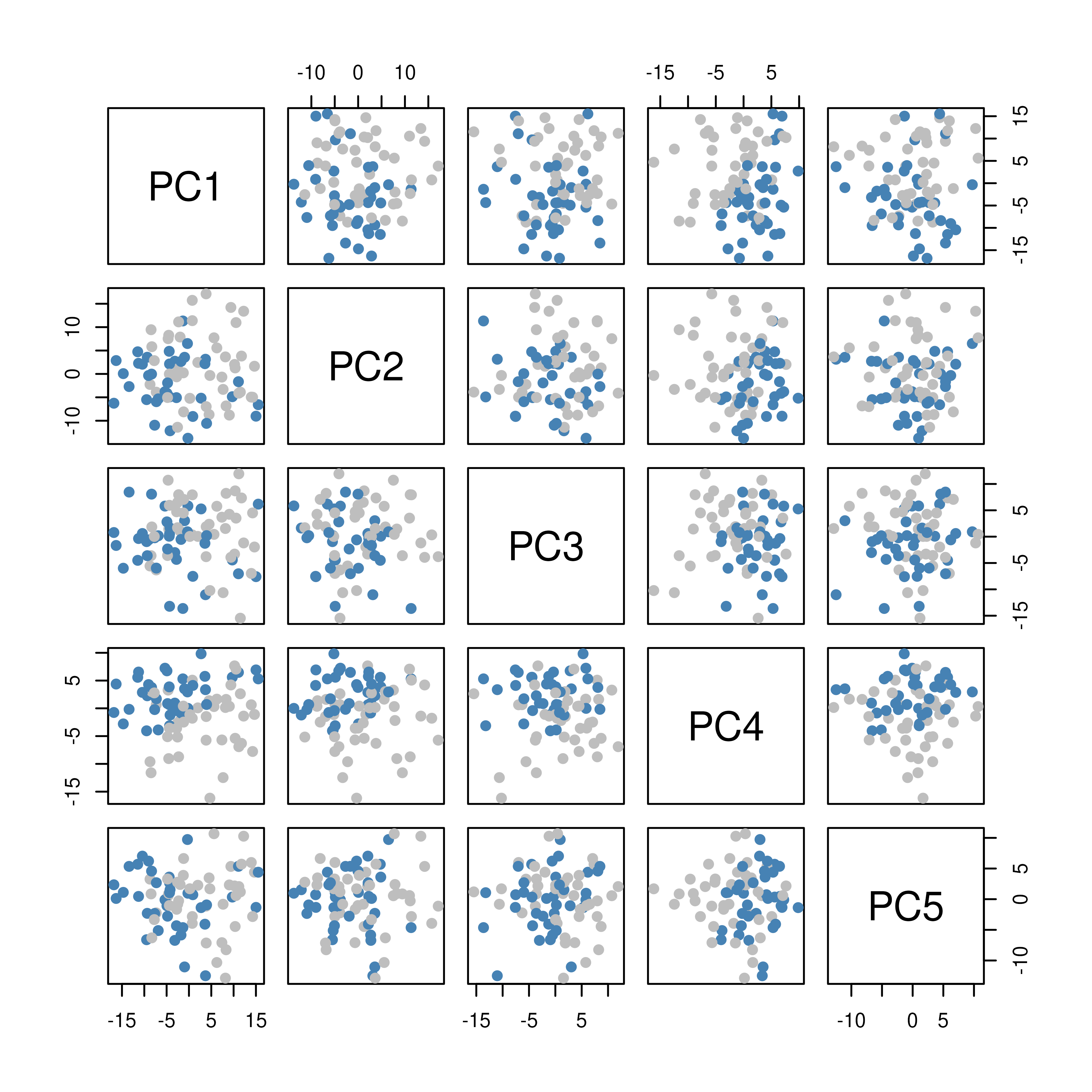

# Biplot of PC1 vs PC2
biplot(PCg)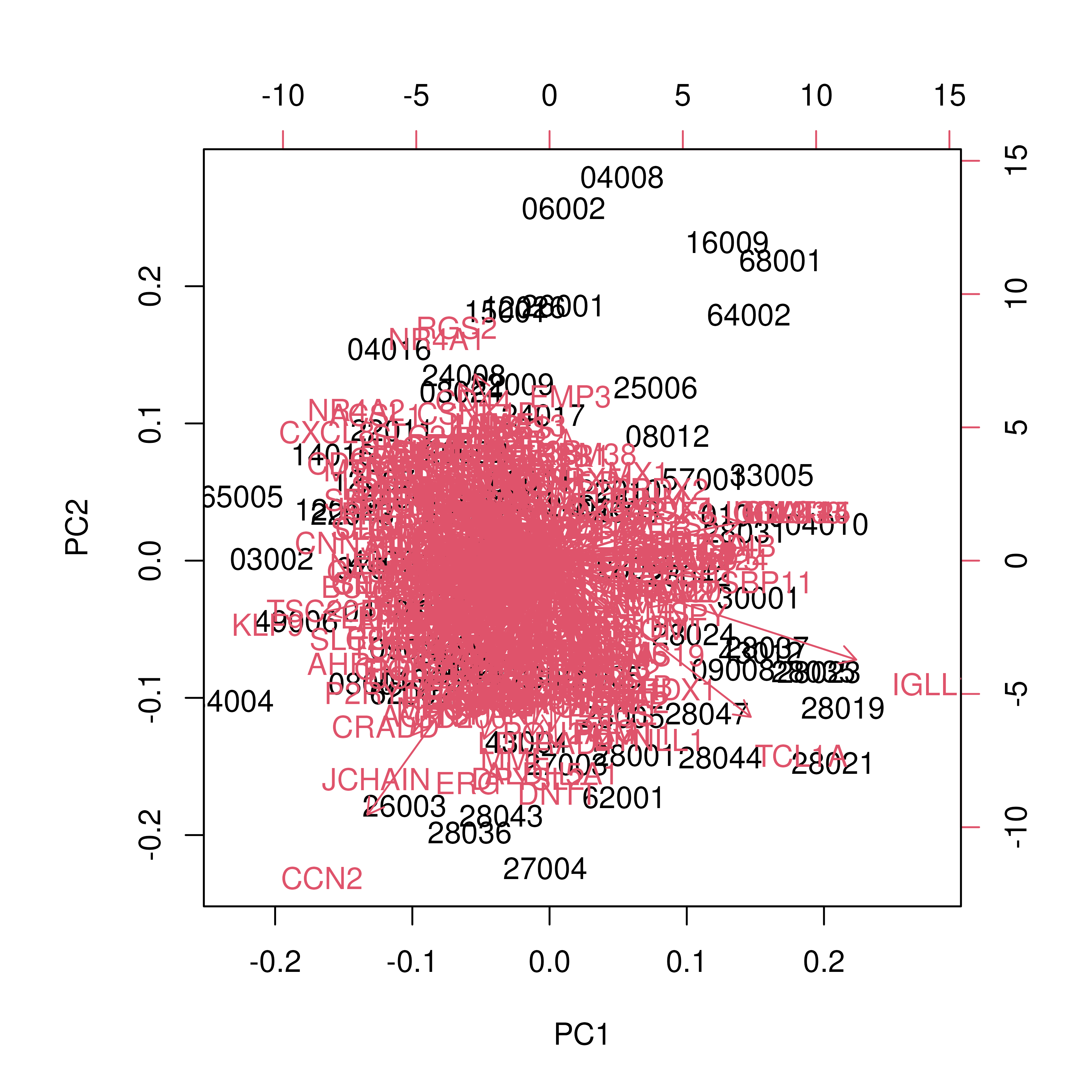

Interpretation:

The heatmap reveals distinct blocks of probes whose expression differs between BCR-ABL1 fusion-positive and fusion-negative samples.

The PCA scatter shows separation (or overlap) of samples by fusion status along the first two principal components, and to a lesser extent, the next three.

In the biplot, probes lying far from the origin along PC1 or PC2 represent genes with the largest loadings, i.e., the greatest contribution to those principal components. Samples positioned similarly share expression patterns in those genes.

Overall, the modest separation in PCA indicates the need for supervised methods to pinpoint the genes most predictive of BCR-ABL1 status.

Train/Test Split and Classifier Training

We split dat_train (ALL) into 60% training and 40% holdout, then train three ML models.

set.seed(2025)                # for reproducibility
n_all <- ncol(dat_train)      # number of ALL samples
train_idx <- sample(n_all, size = floor(0.6 * n_all))
# Training and holdout ExpressionSets
train_eset <- dat_train[, train_idx]
test_eset  <- dat_train[, -train_idx]

In this section, we compare three supervised learning methods using the MLInterfaces framework:

Diagonal Linear Discriminant Analysis (dldaI)
Neural Network (nnetI)
Random Forest (randomForestI)

We will use the MLearn() function, which wraps each algorithm, providing a consistent interface to train, predict, and evaluate models on an ExpressionSet. After fitting, we will use confuMat() to display the confusion matrix, showing the true versus predicted class counts.

We train each model on the first 40 most variable probes from the filtered ExpressionSet (features 1:40 in train_eset).

Diagonal Linear Discriminant Analysis (`dldaI`)

Diagonal LDA assumes each feature is conditionally independent (covariance matrix is diagonal), which can improve stability in high-dimensional, low-sample settings. We use the dldaI interface to fit and evaluate this classifier.

# Train Diagonal LDA on probes 1:40
dlda_mod <- MLearn(
  mol.biol ~ ., # mol.biol ~ . specifies BCR/ABL1 fusion status as the outcome
  train_eset,   # Filtered ExpressionSet
  dldaI,        # dldaI is the diagonal LDA interface
  1:40          # 1:40 selects the first 40 probes
)
#> [1] "mol.biol"

# Print a summary of the fitted model
dlda_mod
#> MLInterfaces classification output container
#> The call was:
#> MLearn(formula = mol.biol ~ ., data = train_eset, .method = dldaI, 
#>     trainInd = 1:40)
#> Predicted outcome distribution for test set:
#> 
#> BCR/ABL     NEG 
#>       3       4

# Display the confusion matrix (true vs predicted)
cm_dlda <- confuMat(dlda_mod)
cm_dlda
#>          predicted
#> given     BCR/ABL NEG
#>   BCR/ABL       3   1
#>   NEG           0   3

# Accuracy of Diagonal LDA
acc_dlda <- sum(diag(cm_dlda)) / sum(cm_dlda)
cat("Accuracy:", sprintf("%.2f%%", acc_dlda * 100))
#> Accuracy: 85.71%

Neural Network (`nnetI`)

A single hidden layer neural network can capture non-linear relationships. We use the nnetI interface with default parameters plus:

size = 5: number of hidden neurons
decay = 0.01: weight-decay regularization
MaxNWts = 2000: maximum allowed number of weights

# Neural Network (nnetI)
nn_mod <- MLearn(
  mol.biol ~ ., 
  train_eset, 
  nnetI, 
  1:40, 
  size=5, 
  decay=0.01, 
  MaxNWts=2000
)
#> [1] "mol.biol"
#> # weights:  1781
#> initial  value 31.210991 
#> iter  10 value 19.645950
#> iter  20 value 12.779243
#> iter  30 value 5.459003
#> iter  40 value 1.841191
#> iter  50 value 1.334631
#> iter  60 value 1.133200
#> iter  70 value 0.875814
#> iter  80 value 0.704137
#> iter  90 value 0.625722
#> iter 100 value 0.610470
#> final  value 0.610470 
#> stopped after 100 iterations

# Show model summary
nn_mod
#> MLInterfaces classification output container
#> The call was:
#> MLearn(formula = mol.biol ~ ., data = train_eset, .method = nnetI, 
#>     trainInd = 1:40, size = 5, decay = 0.01, MaxNWts = 2000)
#> Predicted outcome distribution for test set:
#> 
#> BCR/ABL     NEG 
#>       5       2 
#> Summary of scores on test set (use testScores() method for details):
#> [1] 0.2948988

# Confusion matrix for Neural Net
cm_nn <- confuMat(nn_mod)
cm_nn
#>          predicted
#> given     BCR/ABL NEG
#>   BCR/ABL       4   0
#>   NEG           1   2

# Accuracy of Neural Net
acc_nn <- sum(diag(cm_nn)) / sum(cm_nn)
cat("Accuracy:", sprintf("%.2f%%", acc_nn * 100))
#> Accuracy: 85.71%

Random Forest (`randomForestI`)

Random forests build an ensemble of decision trees on bootstrapped samples and random feature subsets, offering robust performance with little tuning. We use the randomForestI to fit a random forest model:

# Random Forest (randomForestI)
rf_mod <- MLearn(
  mol.biol ~ ., 
  train_eset, 
  randomForestI, 
  1:40
)
#> [1] "mol.biol"

# Show model summary
rf_mod
#> MLInterfaces classification output container
#> The call was:
#> MLearn(formula = mol.biol ~ ., data = train_eset, .method = randomForestI, 
#>     trainInd = 1:40)
#> Predicted outcome distribution for test set:
#> 
#> BCR/ABL     NEG 
#>       4       3 
#> Summary of scores on test set (use testScores() method for details):
#> BCR/ABL     NEG 
#>   0.524   0.476

# Confusion matrix
cm_rf <- confuMat(rf_mod)
cm_rf
#>          predicted
#> given     BCR/ABL NEG
#>   BCR/ABL       4   0
#>   NEG           0   3

# Accuracy of Random Forest
acc_rf <- sum(diag(cm_rf)) / sum(cm_rf)
cat("Accuracy:", sprintf("%.2f%%", acc_rf * 100))
#> Accuracy: 100.00%

Interpretation: Only the Random Forest achieves perfect separation in the validation samples. This highlights the challenge of discriminating BCR-ABL1 status based solely on the top variable probes and underscores why downstream IPD corrections (for regression inference) remain valuable.

Predictions on ALL Test and Golub

After fitting our classifiers on the training subset of ALL, we now generate predictions on both the ALL holdout test and the Golub B-cell ALL datasets.

# Predict BCR-ABL1 status on ALL test holdout using random forest
all_pred <- MLInterfaces::predict.classifierOutput(rf_mod, test_eset)

# Compare to true labels in test_eset
conf_mat_test <- table(
  Truth    = test_eset$mol.biol,
  Predicted= all_pred$testPredictions
)
conf_mat_test
#>          Predicted
#> Truth     BCR/ABL NEG
#>   NEG           3  16
#>   BCR/ABL      11   2

# Predict BCR-ABL1 status on Golub B-cell ALL
golub_pred <- MLInterfaces::predict.classifierOutput(rf_mod, golub_bALL)

# Summarize prediction counts (no ground truth in Golub)
table(golub_pred$testPredictions)
#> 
#> BCR/ABL     NEG 
#>      25      13

Note: We retain true labels in the ALL test set for later IPD; Golub remains unlabeled.

IPD Inference on Sex Effect

We will now use Inference with Predicted Data (IPD) to estimate the log-odds effect of sex (male vs female) on true BCR-ABL1 status, combining the holdout ALL data with true and predict fusion status (i.e., our labeled data) and the Golub data with the predicted fusion status (i.e., our unlabeled data)

# Build labeled (ALL test) data frame
df_test <- tibble(
  sample = colnames(test_eset),
  set    = "labeled",
  true   = as.integer(test_eset$mol.biol == "BCR/ABL"),
  pred   = as.integer(all_pred$testPredictions == "BCR/ABL"),
  sex    = factor(pData(test_eset)$sex, levels = c("F","M"))
)

# Build unlabeled (Golub) data frame
df_golub <- tibble(
  sample = colnames(golub_bALL),
  set    = "unlabeled",
  true   = NA_real_,
  pred   = as.integer(golub_pred$testPredictions == "BCR/ABL"),
  sex    = factor(pData(golub_bALL)$Gender, levels = c("F","M"))
)

# Combine for IPD
ipd_df <- bind_rows(df_test, df_golub) |> drop_na(sex)

# Classical regression
class_fit <- glm(true ~ sex, "binomial", df_test)
class_df  <- broom::tidy(class_fit) |>
  mutate(method = "Classical")

# Naive regression
naive_fit <- glm(pred ~ sex, "binomial", df_golub)
naive_df  <- broom::tidy(naive_fit) |>
  mutate(method = "Naive")

# IPD logistic regression
ipd_fit <- ipd(
  formula   = true - pred ~ sex,
  method    = "pspa",
  model     = "logistic",
  data      = ipd_df,
  label     = "set",
)
ipd_df  <- tidy(ipd_fit) |>
  mutate(method = "IPD")

# Summarize coefficients
combined <- bind_rows(class_df, naive_df, ipd_df) |>
  mutate(term = recode(term, "sexM" = "Male (vs Female)"))

# Forest plot
ggplot(combined, aes(x = estimate, y = term, color = method)) +
  geom_point(position = position_dodge(width = 0.6)) +
  geom_errorbarh(aes(xmin = estimate - 1.96 * std.error,
                     xmax = estimate + 1.96 * std.error),
                 height = 0.2,
                 position = position_dodge(width = 0.6)) +
  geom_vline(xintercept = 0, linetype = "dashed") +
  scale_y_discrete(limits = rev) +
  scale_fill_manual(values  = c("#1B365D", "#00C1D5", "#AA4AC4")) +
  scale_color_manual(values = c("#1B365D", "#00C1D5", "#AA4AC4")) +
  labs(
    x = "Log-Odds Estimate (95% CI)",
    y = "Covariate",
    title = "Comparison of BCR-ABL1 Model Coefficients",
    color = "Model Type"
  ) +
  theme_minimal()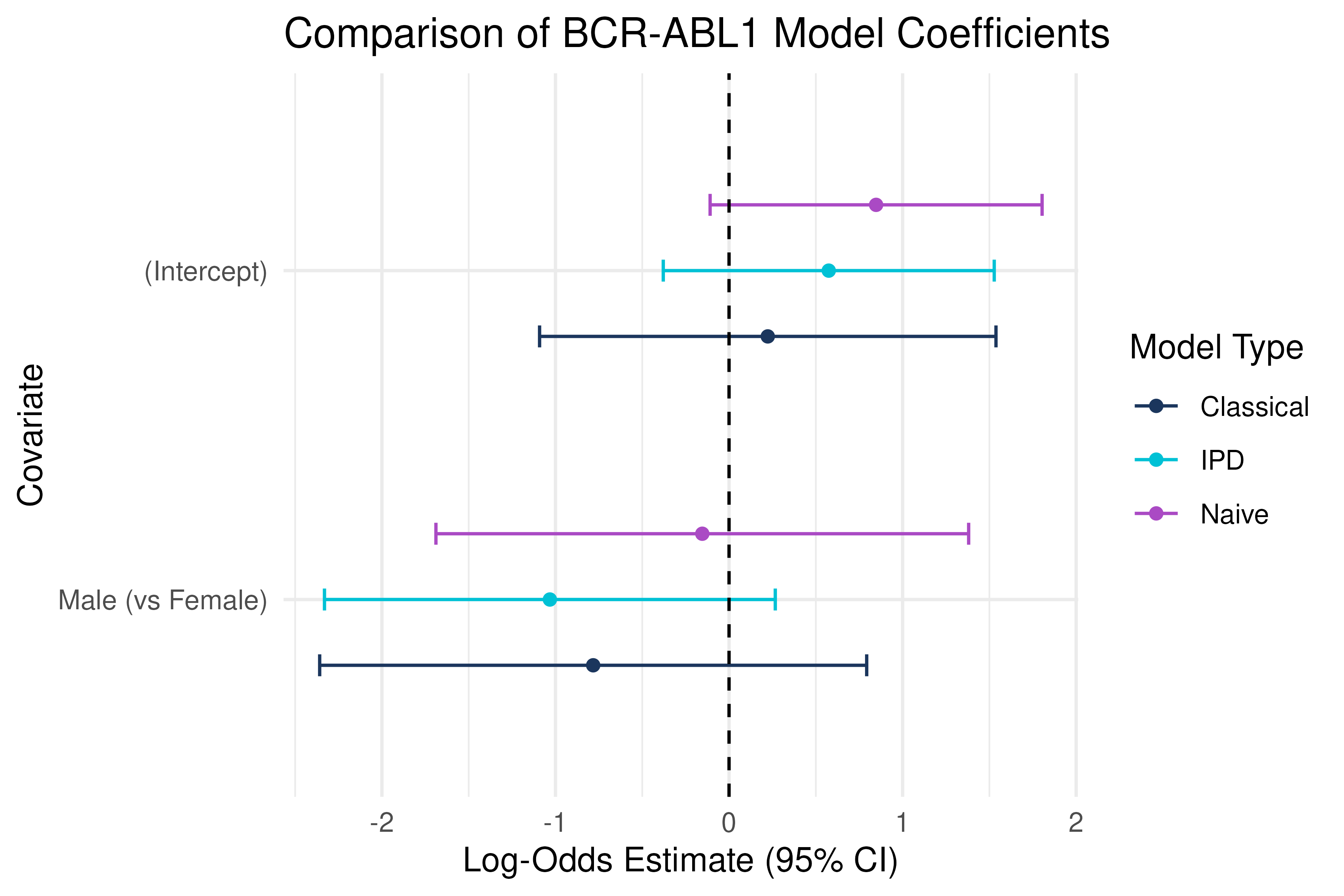

Insight: By treating the ALL test set as labeled and Golub as unlabeled, IPD combines information across cohorts to correct bias and improve precision when estimating the association between BCR-ABL1 status and patient sex.

This is the end of the module. We hope this was informative! For question/concerns/suggestions, please reach out to ssalerno@fredhutch.org

Stephen Salerno

June 24, 2025

Background & Motivation

Datasets Overview

Phenotype Reduction and Feature Filtering

Cross-Platform Probe Harmonization

Exploratory Data Analysis

Train/Test Split and Classifier Training

Diagonal Linear Discriminant Analysis (`dldaI`)

Neural Network (`nnetI`)

Random Forest (`randomForestI`)

Predictions on ALL Test and Golub

IPD Inference on Sex Effect

Unit 03: BCR-ABL Fusion in B-Cell Leukemia

Stephen Salerno

June 24, 2025

Background & Motivation

Datasets Overview

Phenotype Reduction and Feature Filtering

Cross-Platform Probe Harmonization

Exploratory Data Analysis

Train/Test Split and Classifier Training

Diagonal Linear Discriminant Analysis (dldaI)

Neural Network (nnetI)

Random Forest (randomForestI)

Predictions on ALL Test and Golub

IPD Inference on Sex Effect

Diagonal Linear Discriminant Analysis (`dldaI`)

Neural Network (`nnetI`)

Random Forest (`randomForestI`)